Choose the challenges in any order depending on your personal interests and skills. Solving one exercise will possibly need longer than one class !

Challenge: RNA translation¶

Write a script which translates a FASTA file containing RNA sequences to a FASTA file with corresponding amino acid sequences. You find a short and faked FASTA file here

Hint:

use http://siscourses.ethz.ch/python_challenges/codon_table.txt and write Python code to create a dictionary mapping codons to amino acids first.
then write a function which translates a RNA seq to an AA sequence.
then use this function to solve the overall exercise.

Challenge: Formula generator¶

Write a function which takes two mass values and prints all mass formulas consisting of zero or more C, H and / or O where the mass is in the given range. The exact masses are: mass_C = 12.0, mass_H = 1.0078250319 and mass_O = 15.994915.

So for example for the mass range 100.0 to 100.1 the seven formulas H4O6, CH8O5, C2H12O4, C4H4O3, C5H8O2, C6H12O, C8H4 should be printed.

Hints:

you need three nested for loops for this to iterate over all combinations of numbers of C, H and O. The inner code block of those loops computes the mass of the current combination and checks if this fits into the prescribed range.
To minimize the numbers of iterations needed you can estimate the upper bounds of the loops from the upper limit of the mass range.
Further you can estimate a minimal starting value in the most inner loop.

If you solved this introduce some "pretty printing" so that a combination 8 C, 1 H, zero O is displayed as C8H.

Challenge: Simple Spreadsheet¶

We implement spread sheet operations where represent such a sheet as a list of lists.

Learn about Python exceptions first: https://siscourses.ethz.ch/python_dbiol/11_exception_handling.html
Write a function to_float(txt) which converts a string to a float if the string represents a valid float, else return None.
Write a function read_sheet(path) which reads https://siscourses.ethz.ch/python_challenges/data_grouped.csv into a list of lists: every inner list is a row from the sheet. Use Pythons csv module for this.
Write a function pretty_print(sheet) which pretty prints such a sheet, such that all columns have the same width (e.g. 8).

Write a function fix_invalid_numbers which replaces non float entries in a sheet by None values. Use pretty_print to check your results.
Write a function extend_rows which extends all rows of the sheet with None values such that rows have the same length. Again use pretty_print to check your result.
Write a function strip_of_first_column which strips of the first columm of the sheet.
Write a function compute_average(values) which takes a list containing numbers and / or None values. Ignore None for computing the average and return None if there are no valid numbers in the given list.
Combine all functions to load data, fix the sheet, strips of the group column and then compute column-wise averages.

Extension.¶

Learn about defaultdict in Python collections module.
Use a defaultdict(list) to split up the given sheet based on the first column. So the final dictionary should map a group name to a sheet.
Create a new sheet: fist column is group identifier, next columns are column-wise averages of the corresponding "sub-sheet".
Pretty print your result

Challenge "random motion"¶

Quick intro into Python plotting¶

First make sure to install matplotlib and numpy if needed.

import numpy as np
from matplotlib import pyplot

x = np.linspace(0, 2* np.pi, 100)   # discretize 0 .. 2pi to 100 points
print(type(x))
print(x)

<class 'numpy.ndarray'>
[ 0.          0.06346652  0.12693304  0.19039955  0.25386607  0.31733259
  0.38079911  0.44426563  0.50773215  0.57119866  0.63466518  0.6981317
  0.76159822  0.82506474  0.88853126  0.95199777  1.01546429  1.07893081
  1.14239733  1.20586385  1.26933037  1.33279688  1.3962634   1.45972992
  1.52319644  1.58666296  1.65012947  1.71359599  1.77706251  1.84052903
  1.90399555  1.96746207  2.03092858  2.0943951   2.15786162  2.22132814
  2.28479466  2.34826118  2.41172769  2.47519421  2.53866073  2.60212725
  2.66559377  2.72906028  2.7925268   2.85599332  2.91945984  2.98292636
  3.04639288  3.10985939  3.17332591  3.23679243  3.30025895  3.36372547
  3.42719199  3.4906585   3.55412502  3.61759154  3.68105806  3.74452458
  3.8079911   3.87145761  3.93492413  3.99839065  4.06185717  4.12532369
  4.1887902   4.25225672  4.31572324  4.37918976  4.44265628  4.5061228
  4.56958931  4.63305583  4.69652235  4.75998887  4.82345539  4.88692191
  4.95038842  5.01385494  5.07732146  5.14078798  5.2042545   5.26772102
  5.33118753  5.39465405  5.45812057  5.52158709  5.58505361  5.64852012
  5.71198664  5.77545316  5.83891968  5.9023862   5.96585272  6.02931923
  6.09278575  6.15625227  6.21971879  6.28318531]

print(x.shape)

(100,)

# apply function on vector to create a new vector:
y1 = np.sin(x)

# apply functions on vectors to create a new vector
y2 = 0.5 * np.cos(x) + 0.5 * np.sin(2 * x)

%matplotlib inline
pyplot.plot(x, y1)
pyplot.plot(x, y2, "r:", label="y2")  # red dots, try "r." and "yo" and "b*" also
pyplot.legend()  # shows label(s) in a box
pyplot.title("y1 and y2")
pyplot.savefig("y1_and_y2.png")
pyplot.show()

Now lets plot a SQUIRCLE:¶

pyplot.figure(figsize=(4, 4))  # quadratic plot

# "time"
t = np.linspace(0, 4*np.pi, 200)

# radius changes over time
x = np.abs(np.cos(t)) ** .5 * np.sign(np.cos(t))
y = np.abs(np.sin(t)) ** .5 * np.sign(np.sin(t))


# formulas for points on a circle with radius r:
#x = r * np.cos(t)
#y = r * np.sin(t)

pyplot.plot(x, y, "g")  # green lines
pyplot.show()

Exercise¶

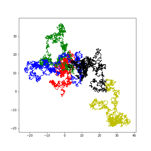
A particle starts at position (0, 0). Then it jumps randomly as follows:

it draws a random angle $\phi$ from $0 \ldots 2\pi$ and a random step size $r$ from the range $0 \ldots 1$.
it updates its position by doing a step of size $r$ in direction $\phi$.

Write a function which does n such iterations and creates two lists of x and y coordinates during these iterations.

Use matplotlib to plot 1000 of such iterations.

Use matplitlib to plot 10000 of such iterations, where every segment of 2000 iterations has a different color.

This is an example using the colors RGBKY in this order:

Challenge: Introduction to Numerical Computations¶

These exercises assume some familiarity with basic calculus. If this is not your cup of tea skip the challenge. The exercises try to give you an idea what the mathematatical research field "numerics" is about.

First read how the bisection method works at https://en.wikipedia.org/wiki/Bisection_method#Iteration_tasks. Use this to find an approximation of $\sqrt{2}$ by looking for a zero of $f(x) = x^2 - 2$.
Use the same function and https://en.wikipedia.org/wiki/Newton%27s_method (here $f'(x) = 2x$) to approximate $\sqrt{2}$. Print a table which shows the values for the first five iterations of both methods.
First look at https://en.wikipedia.org/wiki/Monte_Carlo_method#/media/File:Pi_30K.gif. Now imagine you create a random point in the square. The probability that this point is also in the shown quadrant of the circle is the quotient of the areas of the two objects: $\pi/4$ for the quadrant of the circle and $1$ for the square. So if you create many such random points the fraction of "hits" should approxiamte $\pi/4$. Implement this to compute an approximation of $\pi$ and compute the relative error. (To check such a "hit" use the Pythagorean theorem).
Use the first $n$ terms of https://en.wikipedia.org/wiki/Leibniz_formula_for_%CF%80 to compute an approximation of $\pi$

Challenge: fit data to a given function¶

The following snippet shows how you can determine parameters of a given function to fit to given data:

%matplotlib inline
import numpy as np
import scipy.optimize
import matplotlib.pyplot as pyplot

n_points = 10

x_data = np.arange(n_points)

# we generate artificial data by applying the function f(x) = -0.1 * x^2 + 2 * x + 1
exact_y_data = -.1 * x_data ** 2 + 2 * x_data + 1

# we add some noise with std dev 0.5:
measured_y_data = exact_y_data + 0.5 * np.random.randn(n_points)


def f(x, a, b, c):
    """
    argument x:  vector of values
    argument a:  first parameter to fit
    argument b:  second parameter to fit
    argument c:  third parameter to fit
    
    
    returns:  vector of y values corresponding to parameters a and b
    """
    return a * x * x + b * x + c


# we start with the assumption a = 0, b = 0 and c = 0: 
p_start = np.array([0, 0, 0])

parameters, cov_matrix = scipy.optimize.curve_fit(f, x_data, measured_y_data, p_start)
print(parameters)

pyplot.plot(x_data, exact_y_data, "b", label="exact")
pyplot.plot(x_data, measured_y_data, "b*", label="measured")
pyplot.plot(x_data, f(x_data, parameters[0], parameters[1], parameters[2]), "green", label="fitted")
pyplot.legend(loc=2)  # upper left corner
pyplot.show()

Install numpy, scipy and matplotlib (if not done yet) and reproduce this example. Lookup documentation to understand it.

Logistic growth describes the evolution of a single population in an environment of limited capacity. See https://en.wikipedia.org/wiki/Logistic_function#In_ecology:_modeling_population_growth for details.

Download https://siscourses.ethz.ch/python_challenges/logistic_data.txt and fit the parameters $K$, $P_0$ and $r$ of the corresponding logistic function

$$P(t) = \frac{K P_0 e^{rt}}{K + P_0 \left( e^{rt} - 1\right)}$$

Also create the plots showing the data and the function according to the fitted parameters.
https://siscourses.ethz.ch/python_challenges/logistic_data_multi.txt contains multiple measurements in one single file. Read the data, merge values to $t$ and $P(t)$ vectors and run the fitting again. Hint: the choice of start values for the parameters makes a difference.
Try to automate the downloads using https://pymotw.com/3/urllib.request/index.html, alternatively install requests which is easier to use.

Challenge: Hangman game¶

Implement the Hangman-Game:

the computer knows a secret word
you have to guess letters from the word until the word is disclosed
after every wrong guess the computer informs you about the number of wrong guesses up to now, you loose after 10 wrong guesses
before you enter a guess the computer tells what you disclosed up to now by showing the secret word where a * is displayed for not yet guessed letters.

Exercise:

Below is a template to start. The bodies of the functions are empty, fill them up so that the final program works. The multi line strings you see serve as comments and describe how the functions should work.
Extend it so that the user is allowed to input .. In this case the game should stop.
First code kata: only keep the functions from you solutions and try to re-implement play_game without cheating.
Second code kata: implement the full solution.

Comment: Code katas are exercises where you are asked to re-implement an already known solution starting with a blank or incomplete script. Only lookup the known solution if you get stuck. Repeat this until you don't need to cheat. Make a pause between before the first kata and inbetween kata iterations.

From Wikipedia (https://www.wikiwand.com/en/Kata_(programming)): A code kata is an exercise in programming which helps programmers hone their skills through practice and repetition. The term was probably first coined by Dave Thomas, co-author of the book The Pragmatic Programmer,[1] in a bow to the Japanese concept of kata in the martial arts. As of October 2011, Dave Thomas has published 21 different katas.[2]

By the way: I highly recommend the book https://www.wikiwand.com/en/The_Pragmatic_Programmer !

def print_guessed(word, user_inputs):
    """
    word:  a string holding the secret word
    use_inputs:  a list of letters, collecting the user inputs
    returns: None
    
    this function prints the word letter by letter showing
    unguessed letters as "*"
    
    So the function might show "P Y * * O N" if the word is "PYTHON" and
    the user_input is ["O", "N", "P", "X", "E", "Y"]
    """
    
    
def count_guessed(word, user_inputs):
    """
    word:  a string holding the secret word
    use_inputs:  a list of letters, collecting the user inputs
    
    returns: the number of letters in "word" appearing in "user_inputs".
    """
    
    
def ask_new_guess(user_inputs):
    """
    user_inputs: list of letters already input by user
    returns: new guess from user in upper case
    
    asks until the user provids a new guess, if he repeats a
    previous guess a message is displayed and the user is
    asked again. Same happens if user inputs empty string
    or more than one character
    """
    

def play_game(secret_word):
    user_inputs = []
    guesses_left = 5

    while True: 
        
        print_guessed(secret_word, user_inputs)

        guess = ask_new_guess(user_inputs)
        user_inputs.append(guess)
        
        if guess not in secret_word:
            guesses_left -= 1
            print("WRONG ! %d guesses left !!!" %  guesses_left)
            if guesses_left == 0:
                print("GAME OVER ! THE WORD IS", secret_word)
                break

        print()
        letters_guessed = count_guessed(secret_word, user_inputs)
        if letters_guessed == len(secret_word):
            print("YOU GOT IT !")
            break
            
import random
secret_words = ["notebook", "pythoncourse"]

secret_word = secret_words[random.randint(0, len(secret_words) - 1)].upper()

play_game(secret_word)

Challenge: Phone number data base¶

Write a phone book application. If you start the program the user if asked if he wants to add an new name + phone number or if he wants to lookup an existing phone number. Store the data provided by the user in a csv file so if you restart the program the already entered data will not be lost. So the interaction with the program could look like this:

 PHONEBOOK v1.0
 ==============

 Already 3 entries in the phone book

 Please choose:

     1: add a new entry
     2: lookup a number
     3: show all entries
     0: exit

 Your choice: 1

 Ok, please enter a name: Julian
 And the phone number   : +41 2342 2342

 PHONEBOOK v1.0
 ==============

 Already 4 entries in the phone book

 Please choose:

     1: add a new entry
     2: lookup a number
     3: show all entries
     0: exit

Write functions like

def main_menu(phone_book_entries):

def submenu_add_entry(phone_book_entries): 

def submenu_lookup_entry(phone_book_entries):

etc.

Discard invalid input.

Suggestions:

Either you use a dictionary for lookup or lists. The second approach would allow you to make a lookup which ignores special characters like spaces or . in a name and would ignore the case of the letters.
If you start and the phone book is empty you can use import os and then os.path.exists(..) (use google for futher details) to check if there is already an phone book file or not.
This is a good starting point to learn about object oriented programming. You find an introduction here: https://siscourses.ethz.ch/from_scription_to_professional_software_development/#_object_oriented_programming, implement classes Address and AddressBook to solve this challenge

Challenge: Tic Tac Toe¶

The idea is that two users can place X and O in alternating order by providing coordinates like A2 (for the first row and second column).

A user is not allowed to overwrite a taken field and the computer should detect if X or O wins.

You can represent a 3 times 3 board by nested list like board = [[" ", " ", " "], [" ", " ", " "], [" ", " ", " "]] for the empty board at the beginning.

To get started:

Write a function ask_position which asks the user for a pair like A2. Ask again if position is out of range or else invalid.
Write a function position_to_coordinates(position). Which e.g. transforms A2 to the row / column coordinates (0, 1)
Write a function which asks the user to place a X or O to given coordinates until he chooses a free field. So this could be def place(symbol, board): which then returns the updated board.
Write a function which prints the board nicely as def print_board(board):.
Write a function which checks if a given board represents a winning state like def check_winner(board) which returns X or O or None.

For check_winner you could for example check if you find a row where all values are the same, than the first value of this row would be the result. Same for columns and the two diagonals.

Very advanced: implement the idea of https://makezine.com/2009/11/02/mechanical-tic-tac-toe-computer/ to let the computer play against you !

Challenge: Fetch CHF exchange rates from a web service¶

The following snippet demonstrates how to fetch exchange rate EUR to X for a given date using a so called "web service".

import json
import urllib.request

url = "http://api.fixer.io/2014-01-03"
response_bytes = urllib.request.urlopen(url).read()
print(response_bytes)

b'{"base":"EUR","date":"2014-01-03","rates":{"AUD":1.5156,"BGN":1.9558,"BRL":3.2373,"CAD":1.4468,"CHF":1.2309,"CNY":8.2569,"CZK":27.525,"DKK":7.4586,"GBP":0.83045,"HKD":10.573,"HRK":7.628,"HUF":298.66,"IDR":16533.0,"ILS":4.7749,"INR":84.802,"JPY":142.46,"KRW":1438.7,"LTL":3.4528,"MXN":17.821,"MYR":4.476,"NOK":8.3585,"NZD":1.6434,"PHP":60.892,"PLN":4.1658,"RON":4.4879,"RUB":45.139,"SEK":8.8561,"SGD":1.7244,"THB":45.022,"TRY":2.9637,"USD":1.3634,"ZAR":14.439}}'

So the web service returns a (so called) "byte string" which looks like a dictionary (the format is called JSON). To get a "real" dictionary we can use:

import pprint
data_as_dict = json.loads(str(response_bytes, "ascii"))
pprint.pprint(data_as_dict)  # nicer output than a plain print()

Take the code as it is, communicating to web services is a topic on its own. Another example for a webservice is PUG to query data from Pubchem: https://pubchem.ncbi.nlm.nih.gov/pug_rest/PUG_REST_Tutorial.html

Start with this snippet to write a function which determines the EUR to CHF exchange rate for a given year, month and day.
Then create a plot for the CHF to EUR exchange for the first of every month starting with 1st of january 2015 until today.
Write a function which determines the average exchange rate for a given month. (You remember the leap year computation exercise ?)
Create a plot for the monthly averages.

Challenge: A simple sorting algorithm¶

Implement selection sort to sort a list of numbers. This is the strategy of this algorithm:

Start with index 0 and find the position of a minimal value in the list starting with index 0. Swap the values at both positions.
Go on with index 1 and find the position of a minimal value in the list starting with index 1. Swap the values at both positions.
Go on with index 2 and find the position of a minimal value in the list starting with index 2. ...
.. and so on

So for a list [2, 5, 1, 4, 3] the result of step 0 is [1, 5, 2, 4, 3], the result of step 1 is [1, 2, 5, 4, 3], then [1, 2, 3, 4, 5].

Reproduce and exercise this procedure with pen and paper.
Start with a function min_position(li, start_at) which computes the position of the minimal value staring at the given position start_at.
Then implement a funcion step(i, li) which perfoms step i for the given list (look up the position with min_position(i + 1, li) then swap values at i and the computed position)
Write a loop which performs step(0, li) up to step(len(li) - 1, li)
Test your program for many inputs including empty lists and lists with only one element.

Challenge: Decrypt a substitution cipher¶

Download the encrypted file https://siscourses.ethz.ch/python_dbiol/data/encoded.txt. The text was encoded by a "simple substitution cipher" as described at https://en.wikipedia.org/wiki/Substitution_cipher#Simple_substitution. The cipher kept space characters as space characters.

To break the cipher we make use of the fact that letters occur with different frequencies in texts. This distribution depends on the actual language.

We assume that the letters in English texts ordered by their frequency are etaonhisrldwugfycbmkpvjqxz. So e is the most common character, t the second common character and so on. (This ordering is not fixed but depends on the text corpus used, so you will find slightly modified version on the Internet).

So if a simple substitution cipher maps e to a we should see that a occurs most often in the encrypted text (given that the original text was in English and that the encrypted text is long enough).

To decode the text:

first order the letters from the encoded text by their frequency
then construct a dictionary to map the characters from the given text to their most probable counterpart
and finally use this to decode the text.

The decoding will not be perfect but you should recognize English words and might refine the constructed dictionary manually to improve the result.

Introduction pandas¶

The pandas library support handling of tabular data. In contrast to a numpy matrix every column can have a different type.

pandas allows reading different file formats from different sources:

import pandas as pd

dataset_url = 'http://mlr.cs.umass.edu/ml/machine-learning-databases/wine-quality/winequality-red.csv'
data = pd.read_csv(dataset_url, delimiter=";")
print("shape (rows, cols) is", data.shape)
print("column names are", data.columns)
print(data.head())  # only a few first lines
print(data.tail())  # only a few last lines

shape (rows, cols) is (1599, 12)
column names are Index(['fixed acidity', 'volatile acidity', 'citric acid', 'residual sugar',
       'chlorides', 'free sulfur dioxide', 'total sulfur dioxide', 'density',
       'pH', 'sulphates', 'alcohol', 'quality'],
      dtype='object')
   fixed acidity  volatile acidity  citric acid  residual sugar  chlorides  \
0            7.4              0.70         0.00             1.9      0.076   
1            7.8              0.88         0.00             2.6      0.098   
2            7.8              0.76         0.04             2.3      0.092   
3           11.2              0.28         0.56             1.9      0.075   
4            7.4              0.70         0.00             1.9      0.076   

   free sulfur dioxide  total sulfur dioxide  density    pH  sulphates  \
0                 11.0                  34.0   0.9978  3.51       0.56   
1                 25.0                  67.0   0.9968  3.20       0.68   
2                 15.0                  54.0   0.9970  3.26       0.65   
3                 17.0                  60.0   0.9980  3.16       0.58   
4                 11.0                  34.0   0.9978  3.51       0.56   

   alcohol  quality  
0      9.4        5  
1      9.8        5  
2      9.8        5  
3      9.8        6  
4      9.4        5  
      fixed acidity  volatile acidity  citric acid  residual sugar  chlorides  \
1594            6.2             0.600         0.08             2.0      0.090   
1595            5.9             0.550         0.10             2.2      0.062   
1596            6.3             0.510         0.13             2.3      0.076   
1597            5.9             0.645         0.12             2.0      0.075   
1598            6.0             0.310         0.47             3.6      0.067   

      free sulfur dioxide  total sulfur dioxide  density    pH  sulphates  \
1594                 32.0                  44.0  0.99490  3.45       0.58   
1595                 39.0                  51.0  0.99512  3.52       0.76   
1596                 29.0                  40.0  0.99574  3.42       0.75   
1597                 32.0                  44.0  0.99547  3.57       0.71   
1598                 18.0                  42.0  0.99549  3.39       0.66   

      alcohol  quality  
1594     10.5        5  
1595     11.2        6  
1596     11.0        6  
1597     10.2        5  
1598     11.0        6

print(data.info())

<class 'pandas.core.frame.DataFrame'>
RangeIndex: 1599 entries, 0 to 1598
Data columns (total 12 columns):
fixed acidity           1599 non-null float64
volatile acidity        1599 non-null float64
citric acid             1599 non-null float64
residual sugar          1599 non-null float64
chlorides               1599 non-null float64
free sulfur dioxide     1599 non-null float64
total sulfur dioxide    1599 non-null float64
density                 1599 non-null float64
pH                      1599 non-null float64
sulphates               1599 non-null float64
alcohol                 1599 non-null float64
quality                 1599 non-null int64
dtypes: float64(11), int64(1)
memory usage: 150.0 KB
None

example = data.head()
print(example.shape)
print(example)

(5, 12)
   fixed acidity  volatile acidity  citric acid  residual sugar  chlorides  \
0            7.4              0.70         0.00             1.9      0.076   
1            7.8              0.88         0.00             2.6      0.098   
2            7.8              0.76         0.04             2.3      0.092   
3           11.2              0.28         0.56             1.9      0.075   
4            7.4              0.70         0.00             1.9      0.076   

   free sulfur dioxide  total sulfur dioxide  density    pH  sulphates  \
0                 11.0                  34.0   0.9978  3.51       0.56   
1                 25.0                  67.0   0.9968  3.20       0.68   
2                 15.0                  54.0   0.9970  3.26       0.65   
3                 17.0                  60.0   0.9980  3.16       0.58   
4                 11.0                  34.0   0.9978  3.51       0.56   

   alcohol  quality  
0      9.4        5  
1      9.8        5  
2      9.8        5  
3      9.8        6  
4      9.4        5

example[["pH", "quality"]]

very_good_wines = data[data["quality"] >= 7]
print(very_good_wines.shape)
very_good_wines.head()

(217, 12)

print(very_good_wines["alcohol"].min())
print(very_good_wines["alcohol"].mean())
print(very_good_wines["alcohol"].max())

9.2
11.5180491551
14.0

groupwise_min_values = data[["quality", "alcohol"]].groupby(["quality"]).min()

groupwise_min_values

very_good_wines.to_csv("good_wines.xlsx")

Challenge: very quick intro into machine learning with scikit-learn¶

Preparation: install "pandas" and "scikit-learn".

We can separate learning problems in a few large categories:

supervised learning, in which the data comes with additional attributes that we want to predict. This problem can be either:
- classification: samples belong to two or more classes and we want to learn from already labeled data how to predict the class of unlabeled data.
- regression: if the desired output consists of one or more continuous variables, then the task is called regression.
  
  An example of a regression problem would be the prediction of the length of a salmon as a function of its age and weight.
unsupervised learning in which the training data consists of a set of input vectors x without any corresponding target values.

Examples:

classification: Spam filter, handwritten digit recognition
regression: predict the length of a salmon as a function of age and weight
unsupervised learning: PCA, clustering

For the most cases the learning data is aranged as a feature matrix. Per learning example we use one row, and the data in every row is called a feature vector, the columns of the matrix are the features. For supervised learning we also need a vector of labels which has as much entries as the feature matrix rows.

Example:

import pandas as pd
dataset_url = 'http://mlr.cs.umass.edu/ml/machine-learning-databases/wine-quality/winequality-red.csv'
data = pd.read_csv(dataset_url, delimiter=";")
data["good_quality"] = data["quality"] >= 6

data.head()

Here the columns up to "quality" are the features, and the last column is our label vector.

For getting started we start with 2-dimensional feature vectors which makes plotting easier.

For this we create random points with x and y coordinates in [-1.5, 1.5] and points where both coordinates have the same sign are labeled as "True" and others as "False":

%matplotlib inline

import random
from matplotlib import pyplot
import numpy as np
from sklearn.model_selection import train_test_split

# 300 features of 2d coordinates in range -1.5 to 1.5
points = np.random.random((200, 2)) * 3 - 1.5
labels = (points[:, 0] * points[:, 1]) > 0

# we split our data: 2/3 are used for learning the classifier, the other 1/3 is used
# later for an unbiased validation of the classifier:
points_learn, points_eval, labels_learn, labels_eval = train_test_split(points, labels, test_size=0.333)

print("feature matrix shape for learning  :", points_learn.shape)
print("feature matrix shape for evaluation:",points_eval.shape)

print()
print("first 10 feature vectors + labels:")
for (p, l) in zip(points_learn[:10], labels_learn[:10]):
    print(p, l)

print()
print("red dots are features from class 'False', green dots are from class 'True':")

def plot_examples(points, labels):
    for (p, l) in zip(points, labels):
        x, y = p
        if l:
            pyplot.plot(x, y, "go")
        else:
            pyplot.plot(x, y, "ro")
    pyplot.grid()

pyplot.figure(figsize=(5, 5))
plot_examples(points_learn, labels_learn)
pyplot.show()

feature matrix shape for learning  : (133, 2)
feature matrix shape for evaluation: (67, 2)

first 10 feature vectors + labels:
[ 0.60330361  1.1371488 ] True
[-1.33078797 -0.28353364] True
[ 0.37217748 -1.29483082] False
[ 0.14559219  0.62857116] True
[ 0.37752144 -0.12904102] False
[ 0.14514231 -0.84177145] False
[-0.3029923   0.14351204] False
[-1.47032512 -1.07923806] True
[ 0.81342354 -0.04377843] False
[-0.0640219   1.07251983] False

red dots are features from class 'False', green dots are from class 'True':

Now we train a so called "support vector machine" to distinguish both classes:

from sklearn import svm
from sklearn.utils.extmath import cartesian

# we choose a SVM which is often a good algorithm to get started:
learner = svm.SVC(kernel="rbf", C=100)

# we learn from our features and labels:
learner.fit(points_learn, labels_learn)

# we plot for a all points in a regular grid its class color
# so we undestand better what the "decision surface" looks like:
pyplot.figure(figsize=(5, 5))

def plot_data(grid_2d, labels):
    xs = grid[:, 0]
    ys = grid[:, 1]

    pyplot.plot(xs[labels == 0], ys[labels == 0], "r.", alpha=.2)
    pyplot.plot(xs[labels == 1], ys[labels == 1], "g.", alpha=.2)

x_grid = np.linspace(-1.5, 1.5, 51)
y_grid = np.linspace(-1.5, 1.5, 51)
grid = cartesian((x_grid, y_grid))
pred_labels = learner.predict(grid)

plot_data(grid, pred_labels)

# and we overlay this plot with our training data:
plot_examples(points_learn, labels_learn)

Exercise:

repeat the code examples
try other values for the "C" parameter (eg 1, 0.1 and 1000)
try other classifiers from the scikit learn website, eg "random forests" and "linear svm" or other kernels than "rbf".

To evaluate our classifier we use the points_eval and labels_eval data.

NEVER EVALUATE A CLASSIFIER WITH TRAINING DATA, ALWAYS KEEP A PART OF YOUR DATA AS EVALUATION DATA

TP = True positives (classified as positive, and indeed "positive")
TN = True negatives
FP = False positives (classified as positives, but "negative" in reality)
FN = False negatives

precision: fraction of positive examples among all positive classifications (TP / (TP + FP))
recall   : fraction of positive classified features among all positive features (TP / (TP + FN))

F1       : weighted combination of precision + recall

from sklearn.metrics import classification_report, confusion_matrix

labels_predicted = learner.predict(points_eval)

M = confusion_matrix(labels_eval, labels_predicted)
TN, FN = M[0, :]
FP, TP = M[1, :]

print("True negatives :", TN)
print("True positives :", TP)
print("False negatives:", FN)
print("False positives:", FP)
print()

print(classification_report(labels_eval, labels_predicted))

True negatives : 25
True positives : 37
False negatives: 1
False positives: 4

             precision    recall  f1-score   support

      False       0.86      0.96      0.91        26
       True       0.97      0.90      0.94        41

avg / total       0.93      0.93      0.93        67

import pandas as pd
dataset_url = 'http://mlr.cs.umass.edu/ml/machine-learning-databases/wine-quality/winequality-red.csv'
data = pd.read_csv(dataset_url, delimiter=";")
data["good_quality"] = data["quality"] >= 6

data.head()

from sklearn.ensemble import RandomForestClassifier

features = data.iloc[:, :11]
features -= features.mean()
features /= features.std()

labels = data.iloc[:, 12]
feat_learn, feat_eval, labels_learn, labels_eval = train_test_split(features, labels, test_size=0.333)

learner = RandomForestClassifier()
learner.fit(feat_learn, labels_learn)

labels_predicted = learner.predict(feat_eval)

M = confusion_matrix(labels_eval, labels_predicted)
TN, FN = M[0, :]
FP, TP = M[1, :]


print("True negatives :", TN)
print("True positives :", TP)
print("False negatives:", FN)
print("False positives:", FP)
print()

print(classification_report(labels_eval, labels_predicted))

True negatives : 201
True positives : 210
False negatives: 53
False positives: 69

             precision    recall  f1-score   support

      False       0.74      0.79      0.77       254
       True       0.80      0.75      0.77       279

avg / total       0.77      0.77      0.77       533

Further resources: the online documentation of scikit-learn at http://scikit-learn.org/stable/documentation.html offers very good explanations and code examples for machine learning in general and specific algorithms

Challenge: Recursion¶

We talk about recursion if a function calls itself.

First an example without recursion:

def product(n):
    result = 1
    for i in range(1, n +1):
        result *= i
    return result

print(product(5))

120

This function fulfills the equation product(n) = n * product(n - 1), product(1) = 1. This is a so called "recursive definition".

def product_2(n):
    if n == 1: 
        return 1
    result = product_2(n - 1) * n
    return result

print(product_2(5))

120

To trace this for product_2(3):

result in product_2(3) is result = product_2(2) * 3.
this calls now product_2(2):
result in product_2(2) is result = product_2(1) * 2.
this calls now product_2(1):
which returns 1.
now product_2(2) continues and returns result = 1 * 2
now product_2(3) continues and returns result = 2 * 3 which is 6

I hope you recognize how important the extra handling for n == 1 is, because it breaks the repeated function calls and passes execution back to the caller.

Without such a final case the program would run forever with increasing negative values for n.

Exercise¶

try to understand the explanations
write a recursive function for summing up the numbers 1... n for a given n.
write a recursive functino for summing up numbers in a given list.

Advanced recursion: Quicksort¶

One of the fastest sorting algorithms is called "quicksort". The idea is as follows:

I have a list of numbers, say [3, 4, 2, 7, 1, 6].
I choose the first element 3 as a so called pivot element.
I split the given list in numbers smaller the pivot element and numbers larger or equal the pivot element. So I get lists [2, 1] and [4, 7, 6]. The pivot element is not in both lists.
I take now an arbitrary sorting algorithm to sort both lists individually which gives me [1, 2] and [4, 6, 7].
I place the pivot in the middle and join lists and pivot, so I get the sorted list [1, 2, 3, 4, 6, 7].

Exercise¶

repeat the algorithm for some random numerical lists.

The trick now is to use quicksort again in step 4 which makes this procedure recursive:

Pseudo code is:

    quicksort([]) = [] 
    quicksort(li) for len(li) > 0:
        pivot = li[0]
        li1 = elements (except pivot) in li which are < pivot
        li2 = elements (except pivot) in li which are  >= pivot 
        return quicksort(li1) + [pivot] + quicksort(li2)

Now try to implement this using list comprehensions
Benchmark your runtime for random number lists of increasing size and plot a diagram list size vs runtime. (You might use the time function in the time module for measuring execution time`. Then benchmark for already sorted lists.
Compare this with the runtime of the selection sort algorithm we implemented above.

	fixed acidity	volatile acidity	citric acid	residual sugar	chlorides	free sulfur dioxide	total sulfur dioxide	density	pH	sulphates	alcohol	quality
7	7.3	0.65	0.00	1.2	0.065	15.0	21.0	0.9946	3.39	0.47	10.0	7
8	7.8	0.58	0.02	2.0	0.073	9.0	18.0	0.9968	3.36	0.57	9.5	7
16	8.5	0.28	0.56	1.8	0.092	35.0	103.0	0.9969	3.30	0.75	10.5	7
37	8.1	0.38	0.28	2.1	0.066	13.0	30.0	0.9968	3.23	0.73	9.7	7
62	7.5	0.52	0.16	1.9	0.085	12.0	35.0	0.9968	3.38	0.62	9.5	7

	fixed acidity	volatile acidity	citric acid	residual sugar	chlorides	free sulfur dioxide	total sulfur dioxide	density	pH	sulphates	alcohol	quality	good_quality
0	7.4	0.70	0.00	1.9	0.076	11.0	34.0	0.9978	3.51	0.56	9.4	5	False
1	7.8	0.88	0.00	2.6	0.098	25.0	67.0	0.9968	3.20	0.68	9.8	5	False
2	7.8	0.76	0.04	2.3	0.092	15.0	54.0	0.9970	3.26	0.65	9.8	5	False
3	11.2	0.28	0.56	1.9	0.075	17.0	60.0	0.9980	3.16	0.58	9.8	6	True
4	7.4	0.70	0.00	1.9	0.076	11.0	34.0	0.9978	3.51	0.56	9.4	5	False