WARNING: This script is work in progress
Many chapters are still empty or incomplete.
More and more people code nowadays.
Learning to program is becoming increasingly important in many curricula, both at school and at university. In addition, the emergence of modern and easy to learn programming languages, such as Python, is lowering the entry threshold for taking first steps in programming and attracting novices of all ages from various backgrounds.
As such, programming is not a skill mastered by a small group of experts anymore, but is instead gaining importance in general education, comparable to mathematics or reading and writing.
The idea for this book came up whilst working as a programmer and consultant for ETH Zurich Scientific IT Services. Whether it was during code reviews, code clinics or programming courses for students, researchers, or data scientists, we realized that there is a big need among our clients to advance in programming, and to learn best practices from experienced programmers.
Whilst the first steps in programming focus on getting a problem solved, professional software development is about writing robust, reliable and efficient code, programming in teams, and best practices for writing programs spanning more than a few hundred of lines of code.
Although plenty of established books about such advanced topics exist, most of them are comprehensive and detailed, and require programming experience in advanced topics such as object oriented programming. Beyond that, these books often target programmers already making a living from software development.
On the other hand, introductions to the topics we offer exist but fragmented on the internet. Regrettably theses are not collected and offered in one single place and also are not selected and presented uniformly accordingly to our beliefs.
Regrettably, our clients’ motivation to progress is usually constrained by available time, and by other tasks having higher priority. Answers along the lines of "I fully agree that my code would benefit from your suggested changes, but I have no time for this" are no exception. As a result, we often do not recommend existing books, but instead focus on the most important concepts and on pragmatic, efficient and basic instructions to benefit our clients as efficiently as possible in the face of the given constraints.
This book follows this way of thinking. Instead of trying to provide an all-embracing and deep introduction into the principles of professional software development, our attempt is to select topics we regard as being the most important, and to offer sound introductions and explanations to the underlying concepts and principles. The reader should learn enough to get started and be able to dig deeper by learning from more advanced resources. We also attempt to split the book into chapters with minimal interdependence, so that readers can pick parts according to their interests and existing knowledge.
1. About this book
2. The programming process
3. General principles and techniques
4. Clean code
You might not believe it, but the following program is valid Python code and
prints Hello world!:
1
2
3
4
5
6
7
8
9
10
11
12
13
14
15
16
17
18
19
20
21
22
23
24
25
26
27
28
29
30
31
32
33
34
35
36
37
38
39
40
41
42
43 # hello_world.py
(lambda _, __, ___, ____, _____, ______, _______, ________:
getattr(
__import__(True.__class__.__name__[_] + [].__class__.__name__[__]),
().__class__.__eq__.__class__.__name__[:__] +
().__iter__().__class__.__name__[_:][_____:________]
)(
_, (lambda _, __, ___: _(_, __, ___))(
lambda _, __, ___:
bytes([___ % __]) + _(_, __, ___ // __) if ___ else
(lambda: _).__code__.co_lnotab,
_ << ________,
(((_____ << ____) + _) << ((___ << _____) - ___)) + (((((___ << __)
- _) << ___) + _) << ((_____ << ____) + (_ << _))) + (((_______ <<
__) - _) << (((((_ << ___) + _)) << ___) + (_ << _))) + (((_______
<< ___) + _) << ((_ << ______) + _)) + (((_______ << ____) - _) <<
((_______ << ___))) + (((_ << ____) - _) << ((((___ << __) + _) <<
__) - _)) - (_______ << ((((___ << __) - _) << __) + _)) + (_______
<< (((((_ << ___) + _)) << __))) - ((((((_ << ___) + _)) << __) +
_) << ((((___ << __) + _) << _))) + (((_______ << __) - _) <<
(((((_ << ___) + _)) << _))) + (((___ << ___) + _) << ((_____ <<
_))) + (_____ << ______) + (_ << ___)
)
)
)(
*(lambda _, __, ___: _(_, __, ___))(
(lambda _, __, ___:
[__(___[(lambda: _).__code__.co_nlocals])] +
_(_, __, ___[(lambda _: _).__code__.co_nlocals:]) if ___ else []
),
lambda _: _.__code__.co_argcount,
(
lambda _: _,
lambda _, __: _,
lambda _, __, ___: _,
lambda _, __, ___, ____: _,
lambda _, __, ___, ____, _____: _,
lambda _, __, ___, ____, _____, ______: _,
lambda _, __, ___, ____, _____, ______, _______: _,
lambda _, __, ___, ____, _____, ______, _______, ________: _
)
)
)
If you want to understand how this program works, continue reading here.
|
Writing such obfuscated code maybe fun and challenging. It also may increase your reputation as a coding wizard, but you should definitely invest your mental energy better than into writing such code if you want to be regarded as a professional software developer. |
One common rule is You read code more often than you write it. Let it be because you want to find a bug, you want to extend or improve code, or because others want to learn from it.
So always consider that you might want to understand your own code in weeks or months and, as a non-selfish and team oriented programmer, that this is also the case for others.
Another idea behind good code, is that your code should communicate your solutions ideas and concepts. So code not only instructs your computer to solve a problem, but is a means of communication with humans also.
So, write code for humans, not for computers !
What we present and introduce in this chapter should not be considered as hard rules. As for almost all rules reasonable exceptions exist in real life.
4.1. How does clean code look like ?
What are the hallmarks of readable code ? Following principles are the basis for clean code. Although we list a few examples how to realize these principles, more elaborate explanations and techniques will follow in the following sections:
-
Little scrolling needed. To understand how a "unit" in your code works should require no or little scrolling. This e.g. can be supported by writing short functions and by keeping interdependent parts together.
-
Minimal level of indentation: Loops and branches introducing more than two levels of indentation can be hard to understand, especially if they don’t fit on one single page on your screen. Writing functions can circumvent this. This is also mentioned in the Zen of Python. Newspapers having narrow columns follow the same principle: short and many rows are preferred over long and little rows.
-
Clear naming: Well chosen names are always up-to-date with the code and should support understandability of your code and not confuse the reader. Good names also can avoid unneeded comments and thus contribute to shorter code.
-
Directly understandable: This includes avoiding programming tricks which result in short one liners but will require extra mental work when you or others read this. The code layout should also follow your solution strategy.
-
No surprises: As an example names and comments should never contradict your approach or confuse and cause deep wrinkles on the readers forehead.
-
Consistency: Among st other things, naming of variables and functions should be consistent. So either use
indexas a variable name in all places oridx, but not both ! -
Don’t litter: Keeping out-commented lines of code or unused functions in your code only increases code size and decreases understandability. Use a Version Control System instead.
4.2. General comments about code layout
4.2.1. The usefullness of empty lines
Don’t underestimate the effect of using empty lines to structure your code. An empty line separating two blocks of code guides your eye and makes it easier to focus on such a block. So group related fragments together and separate them with single empty lines. But don’t overuse this !
4.2.2. Keep related statements close together.
Try to structure your code in a way that the flow of operations is as linear as possible. Also try to reduce scattering of related operations, such as initializing and using a specific object.
The following example already uses empty lines to structure the code. But operations such as opening the result file and writing to it, as well as initializing lists and appending data, are scattered:
1
2
3
4
5
6
7
8
9
10
11
12
13
14
15
16
17
18 # grouping_bad.py
with open("results.txt", "w") as fh:
filtered_numbers = []
numbers = [2, 4, 6, 8, 9, 10] (1)
results = []
for number in numbers:
if number % 2 == 0:
filtered_numbers.append(number) (2)
else:
break
for number in filtered_numbers:
results.append(number + 1) (3)
results.append(number ** 2)
for result in results:
print(result, file=fh) (4)
| 1 | The actual data we want to process is defined in the middle of the script. |
| 2 | Your eyes have to move up multiple lines to check the initial value and type of filtered_numbers. |
| 3 | Even more lines to scan to find the initial value and type of results. |
| 4 | You have to read the top of the file to check the used file name and opening mode. Opening and writing is scattered over the script. |
The distinct steps
-
define input data
-
filter data
-
compute results
-
write results
are clearly visible in the reordered code now:
1
2
3
4
5
6
7
8
9
10
11
12
13
14
15
16
17
18 # grouping_good.py
numbers = [2, 4, 6, 8, 9, 10] (1)
filtered_numbers = [] (2)
for number in numbers:
if number % 2 == 0:
filtered_numbers.append(number)
else:
break
results = [] (3)
for number in filtered_numbers:
results.append(number + 1)
results.append(number ** 2)
with open("results.txt", "w") as fh: (4)
for result in results:
print(result, file=fh)
| 1 | The data to process now stands out at the beginning of the script. |
| 2 | Initialization of filtered_numbers is now closer to the following
filtered_numbers.append. |
| 3 | Same for results. |
| 4 | The chosen file name and file opening mode are now also close to the usage of the file handle. |
4.2.3. PEP 8
A code style guide gives general advice on how to format your code to improve readability. If all developers involved in a project follow the same style the code is more consistent, and readable for all people involved.
The most important rules of PEP 8 are:
-
Use multiples of four spaces for indentation.
-
Don’t mix tabs and spaces for indentation. Most IDEs and code editors allow automatic conversion, maybe you have to enable this in your editors settings.
-
Only use lowercase letters, underscores and digits for variable and function names. This is also called snake case. E.g.
input_file_folder. For class names use camel case, this means uppercase characters for the first character of words, else lowercase letters. E.g.InputFileHandler. For constants user uppercase characters and underscores, e.g.DAYS_PER_WEEK. -
Use spaces around assignment
=, comparisons like!=and algebraic operations like+. But no spaces around=for named function arguments or declaring functions with default values. -
Use one space after
, -
no spaces after
[or before], same for(and). -
Maximum 79 characters per line. This is often weakened to 99 characters, but not more !
-
Two empty lines between functions and classes, one empty line between methods.
This is an example for non PEP 8 compliant code:
1
2
3
4
5
6
7
8 # non_pep8.py
class adder:
def __init__(self,x,y):
self.x=x
self.y=y
def addNumbers(numberOne,numberTwo):
return numberOne+numberTwo
And this is the same code after reformatting for PEP 8 compliance:
1
2
3
4
5
6
7
8
9
10 # pep8.py
class Adder:
def __init__(self, x, y):
self.x = x
self.y = y
def add_numbers(number_one, number_two):
return number_one + number_two
| As code in a book reads differently than in a code editor, some of the examples in this book are not PEP 8 compliant, e.g. we use often only one empty line to separate function definitions. |
| Use tools like pep8 to check your code from time to time. Some IDEs also indicate PEP 8 violations or offer tools to format your code for PEP 8 compliance. |
4.2.4. Don’t postpone naming decisions and renaming
Don’t postpone choosing good names when you write code the first times. Don’t postpone rename in case names get out of date during development. Not adapting names to introduced changes can turn your names into lies !
4.3. About good names
This chapter introduces some basic rules for good names. Let it be for variables, functions or also classes.
Can you spot the error in the following example ?
1
2
3 # bad_name.py
def compute(a, b):
return a + b
Compare this to the following code where we use expressive names for the function and the variables:
1
2
3 # good_name.py
def rectangle_area(height, width):
return height + width
Giving functions and variables unambiguous names expressing the programmers
intention can reduce the need for comments. You could try to fix the
first example above by adding a comment that compute computes
the area of an rectangle. The second version does not require a
comment, is shorter and directly understandable. So prefer names like
first_names over the_list or fn.
Encoding the unit of a physical quantity in a variable name makes sense to
reduce errors
and to avoid comments. So is time_since_event not the worst name but
time_since_event_in_seconds will be much clearer (if the unit is fixed and
does not change based on other factors).
I use either idx or index as name or part of names in the same project.
This reduces mental mapping and also searching for already used
names. I also use singular vs plural for distinguishing elements and a collection
of elements. E.g. for first_name in first_names:.
Your brain prefers pronounceable names when reading code. So prefer full words over inconsistent abbreviations.
The term "iteration index" is a term you can use in spoken language when
you communicate with humans, thus prefer the variable name iteration_index over
index_iteration.
If you encode the data type of a variable in its name, you have to change the names
as soon as the data type changes. Else your code will cause confusion.
So better use names instead of name_list, or name_to_phone_number instead
of phone_number_dict.
In the olden days, when Fortran 77 was a modern programming language and the length of variable and function names where restricted, the so called Hungarian notation was a commonly used convention how to encode types into names. As said, this was in the olden days.
Why use a_name if name fulfills the same purpose ? Why income_amount if
income is sufficient ? If a spelling error sneaks into a name, fix this instead
of reproducing the same error all over the code, you might want to search for
the name.
Choose names as general as possible. In the improved
example above we could have used def window_area(window_height,
window_width) instead, because this is how we use this function in our current
house construction project. The choice of more general names here make this
function reusable within other projects without modification.
Using window in the names here also introduces noise as the computation here
is not specific to a window, and the computation will also only be correct if
the window is rectangular.
As classes in most cases represent entities, and methods often are considered
as actions, one should try to choose nouns for class names, and verbs for
method names.
For functions verbs should be preferred, but sometimes nouns are also ok.
E.g. we used rectangle_area above and not compute_rectangle_area, as
area = rectangle_area(h0, w0) reads well and adding compute_ would
introduce noise.
A common convention is to use i, j, and k as variable in a counting loop,
names as n and m for natural numbers, eg. for the length of a list, or for
the dimensions of a matrix. This is ok for names of local variables which are
only used within a small range of lines of code.
4.4. Explanatory variables
Introducing extra variables can enhance readability by far. So you can name sub-expressions of larger mathematical formulas, and avoid error prone duplications. If the names are well chosen extra variables introduce extra information for the reader and thus enhance understandability.
The following code assumes that config is a nested dictionary holding the
configuration settings for some data analysis:
1
2
3
4
5
6 # repeated_expressions.py
def analyze(config, data):
eps = config['numerics']['eps']
max_iteration_count = config['numerics']['max_iteration_count']
max_relative_error = config['numerics']['max_relative_error']
...
By introducing a meaningful variable numerics for a repeated sub-expression
we reduce code duplication, thus the probability of typing mistakes. The result
is also more pleasant to read. In case you rename the key for the numerical
parameters section, only one change is required:
1
2
3
4
5
6
7 # with_sub_expressions.py
def analyze(config, data):
numerics = config['numerics']
eps = numerics['eps']
max_iteration_count = numerics['max_iteration_count']
max_relative_error = numerics['max_relative_error']
...
Another example using an explanatory variable to simplify mathematical expressions:
1
2
3
4
5
6
7
8
9
10
11
12 # quadratic_before.py
import math
def solve_quadratic(p, q):
"""solves x^2 + p x + q == 0"""
if p * p - 4 * q < 0:
return None, None
x1 = -p / 2 + math.sqrt(p * p - 4 * q) / 2
x2 = -p / 2 - math.sqrt(p * p - 4 * q) / 2
return x1, x2
assert solve_quadratic(-3, 2) == (2, 1)
The term \$p^2 - 4q\$ has a mathematical meaning and appeared three
times. This is the improved version using a variable determinant:
1
2
3
4
5
6
7
8
9
10
11
12
13 # quadratic_after.py
import math
def solve_quadratic(p, q):
"""solves x^2 + p x + q == 0"""
determinant = p * p - 4 * q
if determinant < 0:
return None, None
x1 = -p / 2 + math.sqrt(determinant) / 2
x2 = -p / 2 - math.sqrt(determinant) / 2
return x1, x2
assert solve_quadratic(-3, 2) == (2, 1)
Literal values like 24 or 60 in the context of time calculations may be
understandable, but the intention of mem_used / 1073741824 requires a comment:
1 mem_used /= 1073741824 # bytes to gb
Using a constant variable for such magic values is the better solution,
especially when such calculations appear multiple times in different
parts of your code. Usually constants are declared at the top of a script
after the import statements.
1
2
3 BYTES_PER_GB = 1073741824
...
mem_used /= BYTES_PER_GB
4.5. About good comments
The less comments you have to write the better. This is a bold statement and the idea of reducing the amount of comments might be contrary to your current coding practice.
The reason for this is that comments can turn into lies if you change your code but don’t adapt your comments. This is also an example for avoidable redundancy.
The trick is to reduce the amount of comments needed by choosing good names and decomposing your code into small functions.
This comment is redundant and describes what we already know:
1 tolerance = tolerance / 60 # divide by 60
But this comment explains the intention:
1 tolerance = tolerance / 60 # seconds to minutes
When writing comments you can be deep in the programming process and comments will appear understandable. Often this is a misjudgement, because your mind is familiar with the current context. So review your comments and consider if you or others will be able to understand them weeks or months later.
Don’t comment your functions by writing comment lines before the def line.
Python offers a better mechanism: If you declare a string after def and before the
first actual statement of the body of the function this string is called
docstring and automatically contributes to Pythons built-in help system:
1
2
3
4
5
6
7
8
9
10
11
12
13
14
15
16
17
18
19
20 # docstring_example.py
def gcd(m, n):
"""computes greatest common divisor of two numbers (1)
args:
m (int) - first number
n (int) - second number
returns:
gcd (int) - greatest common divisor of m and n (2)
"""
while m != n:
if m > n:
m -= n
else:
n -= m
return m
assert gcd(24, 15) == 3 (3)
assert gcd(1024, 17) == 1
help(gcd)
| 1 | First line of docstring |
| 2 | Last line of docstring |
| 3 | Quick checks if function actually works |
And this is the output from help(gcd):
1
2
3
4
5
6
7
8
9
10 $ python docstring_example.py
Help on function gcd in module __main__:
gcd(m, n)
computes greatest common divisor of two numbers
args:
m (int) - first number
n (int) - second number
returns:
gcd (int) - greatest common divisor of m and n
Often we deactivate code by turning it into comments. This is fine for experiments, but unused code should be removed as early as possible. The same holds for unused functions. The idea of Version Control Systems is to track changes of your source code over time and to allow restoring files from older versions.
4.6. About good functions
Functions are fundamental building blocks for larger programs and we already demonstrated the beneficial effects of using functions to avoid comments. Here we discuss a few recommendations for writing good functions additionally to choosing good names.
To decide if a function name is a good name, and if the way you decompose your problem into functions is well chosen, should mainly be done from the callers perspective.
Ask yourself if the code sections calling your functions are readable, and if another function name or other arguments could improve this. Ask yourself also if the way you call and combine your functions appers to be intuitive and straightforward.
The later introduced technique of test driven development supports this practice.
Lets start with an example of a function not doing one thing: The function
check_prime below asks for a number, checks if its prime, prints some output
and returns a result.
1
2
3
4
5
6
7
8
9
10
11
12
13 # multifunc.py
def check_prime():
n = int(input("number to check ? "))
divisor = 2
while divisor * divisor <= n:
if n % divisor == 0:
print("no prime")
return False
divisor += 1
print("is prime")
return True
check_prime()
And this is an improved version:
1
2
3
4
5
6
7
8
9
10
11
12
13
14
15
16
17
18
19
20 # is_prime.py
def is_prime(n): (1)
divisor = 2
while divisor * divisor <= n:
if n % divisor == 0:
return False
divisor += 1
return True
def ask_user_and_check_prime(): (2)
n = int(input("number to check ? "))
if is_prime(n):
print(n, "is prime")
else:
print(n, "is not prime")
assert is_prime(7)
assert not is_prime(8)
assert not is_prime(9)
ask_user_and_check_prime()
| 1 | We extracted a function is_prime which returns a logical
value indicating if the argument n is prime or not. |
| 2 | We renamed check_prime to ask_user_and_check_prime and the function
has now the purpose of the main task. |
Some benefits:
-
is_primeis reusable, the user of this function can decide where the number to check is coming from and if a result should be printed or not. -
is_primebe tested within an automated testing suite. The former version contained a call ofinput, such user interaction makes automated testing difficult.
| The concept of "one thing" is a bit vague and related decisions sometimes require some gut feeling or experience. This concept gets more cleare in combination with the following sections. |
Long functions spanning multiple pages on a screen are hard to understand and require scrolling, whereas short functions are spatially localized and can be grasped easier.
Splitting up code into small functions also introduces more names, and, provided that the names are well chosen, introduces more information for the reader about how the code works and what parts of the code are intended to do.
Another problem introduced by longer functions is that control statements like
if, continue and break result in different execution paths depending on
the input arguments, as demonstrated in the following example:
1
2
3
4
5
6
7
8 def analyze(n):
if n % 2 == 0:
if n > 0:
...
else:
...
else:
...
Here we see different such execution paths for even and odd numbers, and for even numbers we recognize different paths for positive and non-positive numbers.
Implementing the … code parts in separate functions analyze_for_odd_n,
analyze_for_positive_even_n and analyze_for_non_positive_even_n shortens
the function analyze to a few lines and also introduces separate functions
which can be tested independently.
Implementing the … code parts within in analyze directly would result
in one larger function, and testing this
single function would require analysis of all possible paths and how to trigger
them.
This was a simple example, in real life applications understanding all such possible paths can be challenging and sometimes not all of them are understood and tested.
The code of a function should operate on the same level of abstraction. For example:
1
2
3
4
5 def workflow():
configuration = read_configuration()
data = read_data(configuration)
results = process(data, configuration)
write_result(results, configuration)
The other functions then also should follow this principle. E.g.
1
2
3
4
5
6
7
8 def read_data(configuration):
input_path = configuration['input_file']
if input_path.endswith(".csv"):
return read_csv(input_path)
elif input_path.endswith(".xlsx"):
return read_xlsx(input_path)
else:
raise NotImplementedError('no not know how to read {}'.format(input_file))
A function having multiple sections, maybe including comments to separate
and describe the different
sections, like # read data and # prepare data, is a good candidate for
splitting into different functions.
Another common pattern to avoid are so called flag arguments. Such function arguments are usually integers, sometimes strings, which modify the overall behaviour of a function.
This is an example using such a flag argument action
1
2
3
4
5
6
7
8
9 # flag_argument.py
def update(data, item, action):
assert action in (0, 1, 2)
if action == 0:
data['first_name'] = item
elif action == 1:
data['second_name'] = item
elif action == 2:
data['birthday'] = item
Instead we write different functions with appropriate names:
1
2
3
4
5
6
7
8
9 # without_flag_argument.py
def update_first_name(data, item):
data['first_name'] = item
def update_second_name(data, item):
data['second_name'] = item
def update_birthday(item):
data['birthday'] = item
The more arguments a function has, the harder it is to memorize the arguments, their
order and their intention.
This also increases the risk of introducing bugs.
Function calls with many arguments are also hard to read and understand.
A technique to reduce the number of arguments is to group arguments using dictionaries,
as attributes of classes, or using
namedtuple from the standard libraries collections module.
The argument list of the following function is very long:
1
2
3
4
5
6
7
8 # distance_3d_6_args.py
def distance_3d(x0, y0, z0, x1, y1, z1):
dx = x1 - x0
dy = y1 - y0
dz = z1 - z0
return (dx ** 2 + dy ** 2 + dz ** 2) ** .5
distance = distance_3d(1, 2, 3, 3, 2, 1) (1)
| 1 | The function call is hard to understand, especially if function definition and function call are not as close as here. |
If we introduce a new data type Point3D we obtain a function with only two
arguments:
1
2
3
4
5
6
7
8
9
10
11
12 # distance_3d_2_args.py
from collections import namedtuple
Point3D = namedtuple("Point3D", "x y z")
def distance_3d(p1, p2):
dx = p2.x - p1.x
dy = p2.y - p1.y
dz = p2.z - p1.z
return (dx ** 2 + dy ** 2 + dz ** 2) ** .5
distance = distance_3d(Point3D(1, 2, 3), Point3D(3, 2, 1)) (1)
| 1 | The function call now reveals the intention of the arguments. |
Another technique is to use dictionaries to group configuration settings or algorithmic parameters. The drawback is, that your code only documents the available or required keys within the functions implementation, whereas namedtuples or own classes make this more explicit.
The (at the time of writing) upcoming Python 3.7 release introduces data classes which extend the idea of namedtuples and also introduce automatic type checks.
If grouping arguments does not work a function, I recommend to use named function parameters when calling them. This applies also if you use functions from external libraries.
This example from scipy’s documentation demonstrates this:
1
2
3
4
5
6
7
8 from scipy.interpolate import interp1d
import numpy as np
x = np.linspace(0, 10, num=11, endpoint=True) (1)
y = np.cos(-x**2 / 9.0)
f = interp1d(x, y)
f2 = interp1d(x, y, kind='cubic')
| 1 | In numpy 1.14 the function linspace has six arguments, two
are mandatory, the remaining four are optional to override default values.
So choosing named arguments num=11 and endpoint=True here reveals their
intention and is also independent of the arguments order in the definition of
linspace. |
A function without side effects produces always the same result for same arguments, is independent of the environment and also does not change it.
This is the case for purely mathematical functions, but as soon as a function reads from or writes to a file, this criterion is violated. A file which exists on one computer might not exist on another computer, file permissions might be different, etc.
If a function depends on the environment, it might work on one day but not on another day, and if a functions changes the environment, other functions which worked before might now fail. So side effects can introduce some invisible coupling and thus increase complexity which we should keep as low as possible.
Thus functions without side effects are easier to test with unit-tests, easier to understand and debug, and also easier to re-use.
To reduce such side effects:
-
Isolate functions with side effects and keep them small. E.g. avoid functions which interact with the file system, web services or external programs and at the same time perform other operations like checking data for validity or doing some calculations. This overlaps with the concept that a function should only do one thing.
-
Don’t interact with variables outside the functions body. Python has a
globalstatement, but avoid this. While reading only from a global variable is already problematic, this gets even worse if two or more functions communicate over global variables. They are tightly coupled, are hard to re-use in other programs, and are also difficult to understand. If you still feel you need something like global data, look into object oriented programming, the idea of objects is to group such data and operations on it within classes.
Whereas the former ideas also apply for other programming languages, this section is about an issue specific to Python.
Can you guess what the following program computes ?
1
2
3
4
5
6
7 # mutable_default.py
def foo(a=[]): (1)
a.append(1)
return len(a)
print(foo())
print(foo())
Have you been right ?
1
2
3 $ python mutable_default.py
1
2
| 1 | One would assume that a=[] is executed for every call of foo, but
the list here is only created once when Python parses the code and
constructs the code object for this function. So from call to call
this is the same list object.
When you call foo the first time, the list is extended to [1],
after the second call it is [1, 1] and so on. |
Thus foo has a non-obvious side-effect, the chosen default value for a
changes from function call to function call.
Choosing mutable default values for function arguments can introduce
nasty and hardly detectable bugs. Never use mutable default values
like lists, sets, dictionaries. Immutable default values of type
int, float, bool, str, tuple don’t cause this problem. Same
for None.
|
To avoid this issue, replace mutable default values with None and handle this
default value within the function:
1
2
3
4
5
6
7
8
9 # mutable_default_fixed.py
def foo(a=None):
if a is None:
a = []
a.append(1)
return len(a)
print(foo())
print(foo())
Now you get a reproducible result:
1
2
3 $ python mutable_default_fixed.py
1
1
4.7. Consistency
Consistency relates to consistent code style, consistent naming and also to consistent error handling.
Choose a code style for your project and stick to it.
This is important when you develop code in a team but also for one-man projects. Mixing code styles produces a confusing result, and sticking to the same style makes you feel more comfortable reading or extending parts developed by others.
We recommend PEP 8. This is the most often followed style guide for Python code nowadays, and if you get used to it, you find most exising Python code on the internet or from other sources plesant to read.
Beyond that, the more people follow PEP 8, the more consistent Python code gets overall, not only in distinct projects.
| If you work on an existing project which did not follow PEP 8, refuse to mix the existing style with PEP 8. Code with mixed styles looks very inconsistent and confusing. |
For example choose either idx or index as names or part of names all over
your code.
Consistent naming makes life for programmers much easier by reducing searches for details of given names in the source code.
In a former project I had to read and process text input files with different
content. I choose consistent function names like read_site_from_file,
read_source_from_file, check_site, check_source, insert_site_into_db
and insert_source_into_db etc.
Another example: You develop a program requesting data from different web
services. Then consistency would be increased if you use the term fetch
throughout in variable and functions names, but also in comments. Inconsistent
code would mix fetch and similar terms like retrieve or get.
Functions can fail for different reasons. Be consistent to choose a fixed strategy to handle a specific reason.
E.g. assume within our current project some functions have an identifier as
argument. All such functions should either return None if this identifier is
invalid or raise and (e.g.) ValueError exception, but this should not be mixed.
This makes life for you much easier to implement error handilng if you call such functions.
4.8. Minimize indentation
Deep indentation should be avoided, especially if code spans more than a single page on your screen.
Personal anecdote:
I once was asked to optimize some slow code. Printed on paper the code spanned 20 pages without
declaring any single function. Loops and branches were deeply nested and often spanned
multiple pages. After rewriting the code using functions and reducing indentation we could
spot and fix the slow parts within half an hour.
The following example computes the number of real dividers of natural numbers in a given range. "real dividers" means dividers which are not one or the number itself.
1
2
3
4
5
6
7
8
9
10
11
12 # count_dividers.py
def main(n):
number_dividers = {}
for number in range(2, n):
dividers = 0
for divider in range(2, number):
if number % divider == 0:
dividers += 1 (1)
number_dividers[number] = dividers
return number_dividers
print(main(10))
| 1 | This line has maximal indentation of 16 spaces. |
1
2 $ python count_dividers.py
{2: 0, 3: 0, 4: 1, 5: 0, 6: 2, 7: 0, 8: 2, 9: 1}
Now we move the inner two loops into a separate function count_dividers.
1
2
3
4
5
6
7
8
9
10
11
12
13
14
15 # count_dividers_with_function.py
def count_dividers(number):
dividers = 0
for divider in range(2, number):
if number % divider == 0:
dividers += 1 (1)
return dividers
def main(n):
number_dividers = {}
for number in range(2, n):
number_dividers[number] = count_dividers(number)
return number_dividers
print(main(10))
| 1 | This line has maximal indentation by 12 spaces now. |
Pythons break statement only breaks out of the current loop. To break
out of multiple nested loops usually an extra variable tracking the state
of the iterations is required.
The following slightly unrealistic example demonstrates this: for n taking values 5, 10 and 15 it searches for the first pair of natural numbers which multiplied yield n:
1
2
3
4
5
6
7
8
9
10
11
12
13
14
15
16 # multiple_breaks.py
def main():
for n in (5, 10, 15):
found = False
for i in range(2, n):
for j in range(2, n):
if i + j == n:
print(i, j)
found = True (1)
break
if found: (2)
break
main()
| 1 | We need a variable to inform the loop over i that the inner loop
over j found a match |
| 2 | And now we need an extra break here. |
If me move the two nested loops into a separate function, return allows
us to break out much easier:
1
2
3
4
5
6
7
8
9
10
11
12
13 # multiple_breaks_with_return.py
def check(n):
for i in range(2, n):
for j in range(2, n):
if i * j == n:
print(i, j)
return
def main():
for n in (5, 10, 15):
check(n)
main()
So the next time you seed the pattern from the first example, consider to move the affected loops into a separate function.
The following checks if a given number is prime. It raises an exception when the number is not larger than 1.
1
2
3
4
5
6
7
8
9
10
11
12
13
14 # no_early_exit.py
def is_prime(n):
if n >= 1:
divider = 2
while divider * divider <= n:
if n % divider == 0:
return False
divider += 1
return True
else:
raise ValueError("need number >=1")
assert is_prime(17) is True
assert is_prime(14) is False
Checking fist and raising and exception allows us to implement the actual prime check with less indentation:
1
2
3
4
5
6
7
8
9
10
11
12
13
14 # early_exit.py
def is_prime(n):
if n < 1:
raise ValueError("need number >=1")
divider = 2
while divider * divider <= n:
if n % divider == 0:
return False
divider += 1
return True
assert is_prime(17) is True
assert is_prime(14) is False
The same technique applies for if within loops. Instead of
1
2
3 for n in numbers:
if valid(n):
compute(n)
you can check the opposite and use continue to skip the computation:
1
2
3
4 for n in numbers:
if not valid(n):
continue
compute(n)
The visual effect of this technique is more striking if you replace
compute by a longer code section, maybe also containing more loops and branches.
4.9. How to achieve a row length of maximum 79 or 99 characters in Python ?
There are multiple ways to split a long line into multiple shorter lines. To fix the following line, which is longer than the 79 characters recommended by PEP 8 …
1 this_is_a_long_variable = computation_result_long_abc * computation_result_long_def
we can use \ to indicate that the current line will continue with
the next line:
1
2 this_is_a_long_variable = computation_result_long_abc \
* computation_result_long_def
The Python interpreter also ignores line breaks if opening brackets are not closed yet:
1
2 this_is_a_long_variable = (computation_result_long_abc
* computation_result_long_def)
Or
1
2
3
4
5
6
7
8 addresses = [("peter", "muller", "8001", "zurich"),
("tim", "schmid", "8048", "altstetten"),
]
settings = {"numerics" : {"eps": 1e-3,
"max_iter": 1000},
"output_folder: "/tmp/results",
}
This also works for import:
1
2
3 from math import (cos,
sin,
tan)
Another not widely known feature of Python is automatic string concatenation:
1
2
3 text = ("abc" "def"
"ghi")
assert text == "abcdefghi"
which allows us breaking longer strings over multiple lines. The alternative approach using Pythons multi line strings
1
2 text = """abcdefj
ghi"""
introduces unwanted spaces and a \n.
| In case these methods result in expressions spanning multiple lines, it also can be helpfull to use temporary or explanatory variables to increase readability. This applies escpecially for longer expressions, e.g. mathematical formulas. |
5. Git introduction
git is a so called distributed version control system. It supports working on the same code base by a team of developers, but can also be used within one-man projects. The term version control system, also abbreviated as VCS, means that you can track past changes on your files and that you can also restore them or undo previous changes.
git is a kind of time machine for your code. git also allows managing
different versions of your code in the same folder structure. So with git you don’t
need to encode versions into file or folder names anymore. Say good bye to
script_24-12-2017.py and analysis_01_tim_special.py and look forward to a
clean and well organized code base.
|
Often people heard of git in the context of the code repositories
github.com or gitlab.com, but git can be used on a single machine without
any connection to these repositories.
git was released in 2005 by the Linux developer community. They had to replace their existing VCS and found no suitable alternative to manage contributions from hundreds of developers on a huge code base spanning millions of lines.
| git_s command line interface is a complex beast. For daily work you need only a small fraction of the available commands and options. For rare use cases and special solutions to _git related problems search at stackoverflow.com. |
| git was developed to manage source code or other text files as the asciidoc files for this book, but is not suited to manage binary and / or large files of several MB or larger. Look for git annex and git lfs if your code base contains such files. |
5.1. Installing git
-
On Mac OS X: Fetch the installer from https://git-scm.com/download/mac or use homebrew.
-
On Windows: https://git-scm.com/download/windows. If you run the installer make sure to select
Install Git from Git Bash onlywhen asked. Also install notepad++. -
On Linux: Use your package manager, e.g. on
Ubuntuthe command isapt-get install git.
All following instructions are on the command line within a terminal. Windows users should find a program called git bash after successful installation which offers a terminal.
To check if git works:
1
2 $ git --version
git version 2.11.0
The version number shown on your computer might be different, an exact match is not required for our instructions.
We introduce git here on the command line. Most IDEs nowadays implement their own
user interface to interact with git, but they differ. As most solutions on
stackoverflow.com are instructions at the
command line, you should know how to use git in the terminal anyway.
|
5.2. Initial Configuration
The following commands should be issued once after installing git. They set required and
reasonable default values.
Adapt the values for user.name and user.email to your personal data:
1
2 git config --global user.name "Uwe Schmitt"
git config --global user.email "uwe.schmitt@id.ethz.ch"
On Windows you should find a file named .gitconfig in your home folder.
Open this file with a text editor and add the lines:
[core]
editor = 'C:\\Program Files\\Notepad++\\notepad++.exe'
Maybe you have to adapt this if notepad++ is installed in a different
folder, the single quotes and double backslashes are important !
Now run
1 git config --global core.autocrlf true
to configure line handling, more about this below.
You might adapt the the core.editor setting to your preferred editor, the
second setting of core.autocrlf must not be changed:
1
2 git config --global core.editor /usr/bin/nano
git config --global core.autocrlf input
Windows has a encoding for line endings different to the \n used on Mac OS X and Linux.
This can cause problems if you use git within a team where developers use different operating
systems. Without the specific settings for core.autocrlf above, files with
contain the same text will be considered to be different by git because of the
mentioned discrepancy in line endings.
Even if you intend to use git locally only, don’t skip this setting. You probably will forget this when you start to use git for distributed development in the future.
When you run
1 git config --global -e
your configured editor should show up. Don’t modify the shown file, close the editor immediately.
5.3. Fundamental concepts
We introduce a few underlying concepts of git here.
| Not all our explanations below are 100% exact. We omit some deeply technical details and instead prefer abstractions and concepts which help you to learn and understand git for your daily work. |
5.3.1. Patches
A patch is a text snippet which describes the transformation of a given file to a modified version. Usually such patches are created by a computer.
Let’s start with a file before modification
1
2 def rectangle_area(width, height):
return width + height
which we fix and improve to:
1
2
3 def rectangle_area(width, height):
"""computes area of a rectangle"""
return width * height
Then this is the patch describing those changes:
1
2
3
4
5 @@ -1,2 +1,3 @@
def rectangle_area(width, height):
- return width + height
+ """computes area of a rectangle"""
+ return width * height
Lines 3-5 describe the modification: If we remove starting with -
from the first version and add the lines starting with + we get
the modified file.
|
5.3.2. Commits
A commit consists of a single or multiple related patches. The history is an ordered list of commits.
When saying that git is a kind of time machine for your code, this does not work without your contribution: Commits are not created automatically by git, but you have to decide what changes contribute to a commit and to instruct git to create one.
This is an example how such a history looks like. The most recent entry is a the top.
1
2
3
4
5
6
7
8
9
10
11
12 $ git log (1)
commit 3e6696e23eb41b19f4119f8327cd2b9fd5e462c9 (2)
Author: Uwe <uwe.schmitt@id.ethz.ch> (3)
Date: Fri Apr 27 23:56:42 2018 +0200 (4)
fixed upper limit + added docstring (5)
commit 450b10eb8405130a7e9d7753998b0475d68cd1c8 (6)
Author: Uwe <uwe.schmitt@id.ethz.ch>
Date: Fri Apr 27 23:50:22 2018 +0200
first version of print_squares.py
| 1 | git log shows the history of our git history, more about this command later. |
| 2 | This is the latest commit. the long string after commit is the unique commit id. |
| 3 | The commits author. |
| 4 | The commits time stamp. |
| 5 | Every commit has a commit message describing the commit. |
| 6 | This is the commit before the entry we’ve seen above, compare the time stamps ! |
A commit id is a random string consisting of fourty symbols chosen from 0
.. 9 and a .. f. If we use commit ids in git commands, it is usually
sufficient to use the first eight to ten characters to identify the related commit.
And this is the same history, this time including patches:
1
2
3
4
5
6
7
8
9
10
11
12
13
14
15
16
17
18
19
20
21
22
23
24
25
26
27
28
29
30
31
32
33 $ git log -p (1)
commit 3e6696e23eb41b19f4119f8327cd2b9fd5e462c9
Author: Uwe <uwe.schmitt@id.ethz.ch>
Date: Fri Apr 27 23:56:42 2018 +0200
fixed upper limit + added docstring
diff --git a/print_squares.py b/print_squares.py (2)
index 140c0a6..18fce63 100644
--- a/print_squares.py
+++ b/print_squares.py
@@ -1,3 +1,4 @@
def print_squares(n):
- for i in range(1, n):
+ """prints squares of numbers 1 .. n"""
+ for i in range(1, n + 1):
print(i, "squared is", i ** 2) (3)
commit 450b10eb8405130a7e9d7753998b0475d68cd1c8
Author: Uwe <uwe.schmitt@id.ethz.ch>
Date: Fri Apr 27 23:50:22 2018 +0200
first version of print_squares.py
diff --git a/print_squares.py b/print_squares.py
new file mode 100644
index 0000000..140c0a6
--- /dev/null (4)
+++ b/print_squares.py
@@ -0,0 +1,3 @@
+def print_squares(n):
+ for i in range(1, n):
+ print(i, "squared is", i ** 2)
| 1 | git log -p additionally shows the patches related to every commit. |
| 2 | This is where the patch for the latest commit starts. |
| 3 | And this is where the patch for the latest commit ends. |
| 4 | This is a special patch. The /dev/null indicates that the file did not
exist before this commit. We see only added lines in the patch, thus this
commit describes the very first version of print_squares.py. |
You might have several changes in your files, but done for different reasons. Maybe one file was changed to fix a bug and changes in two other files implement a new feature of your software. Good practice is to create two commits for this. The first commit should contain the patches for fixing the bug, the other commit implements the new feature.
Commits should also be small. So in case you program daily, better create commits several times a day instead once a week.
One reason for this is that git e.g. allows undoing a previous commit as a whole, so undoing changes gets difficult if you only want to undo a part of a commit.
Try to separate commits which clean or restructure code, commits which fix bugs and commits adding or changing functionality.
Tasks like "I thought I fixed this bug, let’s find and inspect the related commit", or "What code changes actually implemented the new database scheme" will much easier if you follow these recommendations.
5.3.3. Staging Area / Index
To generate a commit we first must create patches and collect them in the
so called staging area, also named index.
We learn later the git add command which exactly does this.
5.4. Basic Git Hands-On
We introduce now a few git commands in a hands-on session. Please reproduce all steps on your computer. Typing helps to memorize the various git commands.
1
2
3 $ cd (1)
$ mkdir -p tmp/git_intro (2)
$ cd tmp/git_intro (3)
| 1 | An empty cd changes the working directory to your home folder. |
| 2 | We create a folder for the hands-on, the -p also creates the tmp folder if needed. |
| 3 | We cd into this folder. This is now our working directory for the following hands-on. |
To put the current folder under version control, we create a local git repository
using git init.
1
2
3
4
5
6
7
8
9
10
11
12
13
14
15 $ git init . (1)
Initialized empty Git repository in /Users/uweschmitt/tmp/git_intro/.git/
$ ls -al (2)
total 0
drwxr-xr-x 3 uweschmitt staff 96 Jun 2 23:12 .
drwxr-xr-x 37 uweschmitt staff 1184 Jun 2 23:12 ..
drwxr-xr-x 10 uweschmitt staff 320 Jun 2 23:12 .git
$ git status (3)
On branch master
No commits yet
nothing to commit (create/copy files and use "git add" to track)
| 1 | The . refers to the current working directory. The message you see in the following
line will be different on your computer. |
| 2 | The .git folder indicates that the current folder (and all future sub-folders)
are now under version control. This folder contains all data managed by git, e.g.
all commits. Never remove the .git folder ! |
| 3 | git status tells us that the repository is still empty. |
From now on the folder containing the .git directory and all files and
subfolders are under version control.
|
| Never create a git repository within an existing repository. |
We create a file prime_number.py in the current directory with the following content:
1
2
3
4
5
6
7 def is_prime(n):
divisor = 2
while divisor * divisor <= n:
if n % divisor == 0:
return False
divisor += 1
return True
Then we create our first commit:
1
2
3
4
5
6
7
8
9
10
11
12
13
14
15
16 $ git add prime_number.py (1)
$ git status
On branch master
No commits yet
Changes to be committed: (2)
(use "git rm --cached <file>..." to unstage)
new file: prime_number.py
$ git commit -m "first version of prime_number.py" (3)
[master (root-commit) b5f618d] first version of prime_number.py
1 file changed, 7 insertions(+)
create mode 100644 prime_number.py
| 1 | We add the new file to the staging area. |
| 2 | git status tells us that there is a new file in the staging area. |
| 3 | We create a commit, after -m you see the commit message we choose for this commit.
Just issuing git commit would open the configured editor where we can enter and save the commit message. |
1
2 $ git log
fatal: your current branch 'master' does not have any commits yet
Now we add a new function to prime_number.py:
1
2
3
4
5
6
7
8
9
10 def is_prime(n):
divisor = 2
while divisor * divisor <= n:
if n % divisor == 0:
return False
divisor += 1
return True
def primes_up_to(n):
return [i for i in range(2, n + 1) if is_prime(i)]
And a new file test_prime_number.py in the same folder:
1
2
3
4 from prime_number import *
up_to_11 = primes_up_to(11)
assert up_to_11 == [2, 3, 5, 7, 11], up_to_11
git diff tells us differences relative to the last commit:
1
2
3
4
5
6
7
8
9
10
11
12 $ git diff
diff --git a/prime_number.py b/prime_number.py
index 75e70ec..4b54780 100644
--- a/prime_number.py
+++ b/prime_number.py
@@ -5,3 +5,6 @@ def is_prime(n):
return False
divisor += 1
return True
+
+def primes_up_to(n):
+ return [i for i in range(2, n + 1) if is_prime(i)]
and git status shows us that there is a new file not under version control yet:
1
2
3
4
5
6
7
8
9
10
11
12
13
14
15
16
17
18
19
20 $ git status
On branch master
Initial commit
Changes to be committed:
(use "git rm --cached <file>..." to unstage)
new file: prime_number.py
Changes not staged for commit:
(use "git add <file>..." to update what will be committed)
(use "git checkout -- <file>..." to discard changes in working directory)
modified: prime_number.py
Untracked files:
(use "git add <file>..." to include in what will be committed)
test_prime_number.py
1
2
3
4
5
6
7
8
9
10
11
12
13
14 $ git add prime_number.py (1)
$ git add test_prime_number.py (2)
$ git status (3)
On branch master
Changes to be committed:
(use "git reset HEAD <file>..." to unstage)
modified: prime_number.py
new file: test_prime_number.py
$ git commit -m "added new function and test script" (4)
[master cb29a6b] added new function and test script
2 files changed, 7 insertions(+)
create mode 100644 test_prime_number.py
| 1 | We add the patch for the changes in prime_number.py to the staging area. |
| 2 | We add the new file test_prime_number.py to the staging area. |
| 3 | git status now confirms the state of the staging area holding patches related to the two files. |
| 4 | We create a new commit. |
1
2
3
4
5
6
7
8
9
10
11
12
13
14
15
16
17
18
19
20
21
22
23
24
25
26
27
28 $ git show (1)
commit cb29a6b5974ba6a571e12209e18753d480761849
Author: Uwe <uwe.schmitt@id.ethz.ch>
Date: Sat Jun 2 23:13:33 2018 +0200
added new function and test script
diff --git a/prime_number.py b/prime_number.py (2)
index 75e70ec..4b54780 100644
--- a/prime_number.py
+++ b/prime_number.py
@@ -5,3 +5,6 @@ def is_prime(n):
return False
divisor += 1
return True
+
+def primes_up_to(n):
+ return [i for i in range(2, n + 1) if is_prime(i)]
diff --git a/test_prime_number.py b/test_prime_number.py (3)
new file mode 100644
index 0000000..1cac7da
--- /dev/null
+++ b/test_prime_number.py
@@ -0,0 +1,4 @@
+from prime_number import *
+
+up_to_11 = primes_up_to(11)
+assert up_to_11 == [2, 3, 5, 7, 11], up_to_11
| 1 | git show shows the latest commit. We see that this commit contains two patches. |
| 2 | This is the first patch. |
| 3 | And this is the second patch. |
5.4.1. Summary
These are the commands we used up to now:
-
git addto add new or modified files to the staging area -
git commit -m '…'to create the commit. -
git diffshows current changes relative to the last commit. -
git statusshows the current status of the repository. -
git logshows the history of the repository. -
git showto show the latest commit.
5.5. What’s next ?
5.5.1. Other helpfull commands
-
git log --onelineto show a compressed history with one line per commit. -
git diff --cachedto inspect the staging are -
git show COMMIT_IDto show a commit having idCOMMIT_ID. -
git blame FILEshows each line in the givenFILEwith information from -
git resetto empty the staging area in case you added a file unintendedly. -
git commit --amendto add the current staging area to the latest commit. Usefull if you forgot to add some files in the latest commit. the commit which last modified the line.` -
git checkout FILEresets the namedFILEto the latest version. -
git checkout .resets all files and folders in the current working directory to the latest git version. -
git rmto remove files under version control. -
git mvto rename or move files under version control.
5.5.2. The .gitignore file
git status will also show backup files from your editor or .pyc files or
the __pycache__ folder. To ignore such files and folders you can create a
file named .gitignore, usually in the main folder of the repository. My
repositories usually have a .gitingore file including the following lines:
1
2
3 **/*.pyc (1)
**/.*.sw? (2)
**/__pycache__ (3)
| 1 | Ignores all files ending with .pyc in all subfolders (**). |
| 2 | Ignores all files like .primes.py.swp or .primes.py.swo which are
backup files from vim. |
| 3 | Ignores files and folders named __pycache__ in all subfolders. |
-
Also commit the
.gitignorefile to your repository. -
Add all huge or binary files to
.gitignore.
5.6. How to bring existing source code under version control.
git init . also works is the current folder contains existing code. So to introduce
version control for an existing project follow the following instructions:
-
cdto your projects root folder. -
git init . -
git statusand look for files, folders and name patterns you don’t want to add. -
Create a
.gitignorefile to exclude these. -
git add …for all files or folders you want to bring under version control. -
git resetresets the staging area if you added unwanted files or folders. -
git add .gitignore -
git commit -m "initial commit"
5.7. About branches
Branches support maintaining different versions of source code in the same
git repository. Below you see an example showing two branches master
and feature. In the example below, the master branch is
active, and git log will show you commits 3, 2 and then 1.
The files and folders in your git repository will also correspond
to the commits from this branch.
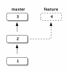
If you checkout (activate) the branch feature your files will correspond to
the commits from the history 4, 2 and 1:
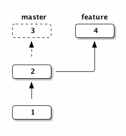
So branches allow switching of files and folders in your repository to manage different versions of your code.
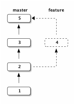
Branches can also be merged. Here we merged feature into master, this created
a new commit 5 combining the changes introduced in commits 3 and 4:
The master branch is the default branch, which we used all the time, and
which you see in the output of git status from the previous hands-on session.
-
Try to keep the
masterbranch clean and working. -
If you implement a new feature create a new branch for this. When development is complete and your changes are tested you can merge this branch back into
master. This also allows bug-fixes in themasteror a dedicated bug-fix branch when the work onfeatureis not completed. -
Use branches for different versions of your software. So you can fix older bugs even if the development proceeded meanwhile. This helps when users don’t want the most current version (could break their applications), but still need a bug-fix.
-
We see later how to use branches if you want to step back in time to inspect your repository some commits ago.
5.7.1. Branching and Merging Hands-On
The following examples are based on the repository we used during the first hands-on session teaching basic git commands.
git branch shows available branches, and the active branch is marked with *:
1
2
3
4
5
6 $ git branch (1)
* master
$ git log --oneline (2)
897d002 added new function and test script
3c6205c first version of prime_number.py
| 1 | We have only one branch in the repository up to now. |
| 2 | This is the current history of the master branch. |
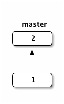
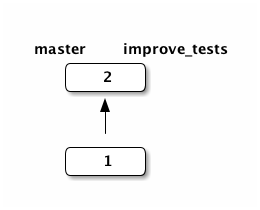
And the following sketch depicts the state of the master repository:
Now we create a new branch:
1
2
3
4
5
6
7
8
9
10
11
12
13
14
15 $ git branch improve_tests (1)
$ git branch (2)
improve_tests
* master
$ git checkout improve_tests (3)
Switched to branch 'improve_tests'
$ git branch (4)
* improve_tests
master
$ git log --oneline (5)
897d002 added new function and test script
3c6205c first version of prime_number.py
| 1 | git branch improve_tests creates a new branch with the given name. |
| 2 | We see now both branches, master is still the active branch. |
| 3 | git checkout improve_tests activates the new branch. |
| 4 | We see both branches again, but the active branch changed. |
| 5 | The new branch still has the same history as the master branch. |
This image reflects the state of our repository: two branches with the same history:
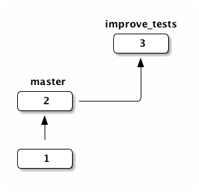
Now we extend the test_prime_numer.py by adding two new lines at the end
of the file:
1
2
3
4
5
6 from prime_number import *
up_to_11 = primes_up_to(11)
assert up_to_11 == [2, 3, 5, 7, 11], up_to_11
assert primes_up_to(0) == []
assert primes_up_to(2) == [2]
Let’s inspect the changes and create a new commit in our new branch:
1
2
3
4
5
6
7
8
9
10
11
12
13
14
15
16
17
18
19
20
21 $ git diff
diff --git a/test_prime_number.py b/test_prime_number.py
index aaf9064..b258c6d 100644
--- a/test_prime_number.py
+++ b/test_prime_number.py
@@ -2,3 +2,5 @@ from prime_number import *
up_to_11 = primes_up_to(11)
assert up_to_11 == [2, 3, 5, 7, 11], up_to_11
+assert primes_up_to(0) == [] (1)
+assert primes_up_to(2) == [2]
$ git add test_prime_number.py
$ git commit -m "improved tests"
[improve_tests 2925e4d] improved tests
1 file changed, 2 insertions(+)
$ git log --oneline
2925e4d improved tests
1d864cd added new function and test script
064a280 first version of prime_number.py
| 1 | These are the two new lines. |
The branch feature_branch now has a third commit and now deviates from the
master branch:
Let’s switch back to master and check test_prime_number.py:
1
2
3
4
5
6
7
8 $ git checkout master (1)
Switched to branch 'master'
$ cat test_prime_number.py (2)
from prime_number import *
up_to_11 = primes_up_to(11)
assert up_to_11 == [2, 3, 5, 7, 11], up_to_11
| 1 | We activate the master branch again. |
| 2 | And we see that the test_prime_number.py script is without the recent
changes we did in the improve_tests branch. |
Next we improve our is_prime function. We handle even values of n first
and then reduce the divisors to odd numbers 3, 5, 7, …:
1
2
3
4
5
6
7
8
9
10
11
12
13
14
15
16 def is_prime(n):
if n == 2:
return True
if n % 2 == 0:
return False
divisor = 3
while divisor * divisor <= n:
if n % divisor == 0:
return False
divisor += 2
return True
def primes_up_to(n):
return [i for i in range(2, n + 1) if is_prime(i)]
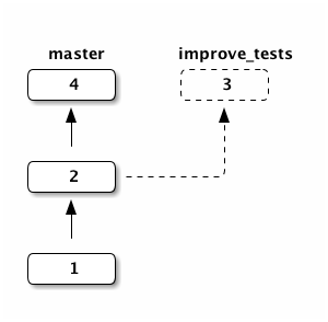
We commit these changes:
1
2
3
4
5
6
7
8
9
10
11
12
13
14
15
16
17 $ git add prime_number.py
$ git commit -m "improved is_prime function"
*** Please tell me who you are.
Run
git config --global user.email "you@example.com"
git config --global user.name "Your Name"
to set your account's default identity.
Omit --global to set the identity only in this repository.
fatal: unable to auto-detect email address (got 'root@f54e1484dc35.(none)')
$ git log --oneline
fatal: your current branch 'master' does not have any commits yet
And this is the current state of the repository:
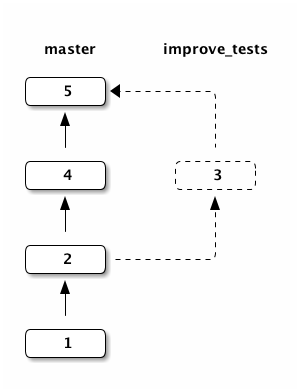
Now we merge the improve_tests branch into master:
1
2
3
4
5
6
7
8
9
10
11
12
13
14
15
16
17 $ git branch (1)
improve_tests
* master
$ git merge improve_tests (2)
Merge made by the 'recursive' strategy.
test_prime_number.py | 2 ++
1 file changed, 2 insertions(+)
$ git log --oneline --graph (3)
* da3a460 Merge branch 'improve_tests'
|\
| * 55c9744 improved tests
* | cef78db improved is_prime function
|/
* 6f98631 added new function and test script
* a52a49e first version of prime_number.py
| 1 | We make sure that master is the active branch. |
| 2 | We merge improve_tests into the active branch. |
| 3 | This shows the history with extra symbols sketching the commits from merged branches.
We also see, that git merge created a new commit with an automatically generated message. |
And this is the current state of our repository:
A so called merge conflict arises when we try to merge two branches with overlapping changes.
In this case git merge fails with an corresponding message, git status also
shows a Unmerged paths section with the affected files.
If you open an affected file you will find sections like
<<<<<<< HEAD
while i < 11:
   j += i
=======
while i < 12:
   j += i ** 2
>>>>>>> branch-a
The two sections separated by marker lines <<<<<< HEAD, ======= and
>>>>>> branch-a show the conflicting code lines. branch-a is here the name
of the branch we want to merge, and as such can differ from merge to merge.
The computer is not able to determine the intended merge of the shown sections, instead human intervention is needed. Thus the users has to edit the file and decide how the code should look like after merging. The markers also have to be removed.
We could e.g. rewrite the example fragment as:
while i < 11:
   j += i ** 2
The full procedure to resolve the merge conflict(s) is as follows:
-
Open a file with an indicated merge conflict in your editor.
-
Find the conflicting sections.
-
Bring the two parts lines between
<<<<<<and>>>>>>to the intended result without the three marker lines. -
If done for all conflicting sections save the file and quit the editor.
-
git add FILE_NAMEfor the affected file. -
Repeat from 1. until you resolved all merge conflicts.
-
git commit(without any message) completes the merge process.
Between the failing git merge and the final git commit your
repository is in an intermediate state. Always complete resolving a merge
conflict, or use git merge abort to cancel the overall merging process.
|
5.8. Remote repositories
Up to now we worked with one local git repository. Beyond that git allows synchronization of different repositories located on the same or remote computers.
Known hosting services such as github.com and gitlab.com manage local git
repositories on their servers and offer a convenient web interface for
additional functionalities supporting software development in a team.
The open-source software gitlab-ce (gitlab community edition) is
the base for the free services at gitlab.com and can be installed
with little effort. This enables teams or organizations to run their
own gitlab instance.
There are different use-cases for remote repositories:
-
You want to share your code. For general availability of your code you can use so called public repositories, for a limited set of collaborators you can use private repositories. Public repositories allow others to implement changes or bug-fixes and offer them as so called merge requests (
gitlab.com) or pull requests (github.com). -
You want work on the same software project in a team.
-
You develop and run code on different machines. A remote repository can be used as an intermediate storage.
-
Last but not least, a remote repository can be used as a backup service.
To reproduce the following examples you need
an account on gitlab.com or github.com. To create an account you have to
provide your email address and your name, after that you should receive an
email containing a link to complete your registration and to set you password.
To setup passwordless connection of the command line git client to your remote repositories, we need a key pair.
Run this in your terminal:
1
2
3
4
5
6 $ test -f ~/.ssh/id_rsa.pub || ssh-keygen -t rsa -P "" -f ~/.ssh/id_rsa.pub (1)
$ cat ~/.ssh/id_rsa.pub
ssh-rsa AAAAB3NzaC1yc2EAAAADAQABAAACAQCeBGRBsNYSD5RBSDFdC (2)
....
....
+w== uweschmitt (3)
| 1 | You already might have created a key pair (e.g. for passwordless ssh
access to other computers). Here we run ssh-keygen only if no such key pair
exists. |
| 2 | This is where the public key starts |
| 3 | And this is where it ends, we ommitted some lines. |
Copy the public key, then
Choose a name and create a project:
-
gitlab.comusers follow read here until '5. Click Create project.' -
github.comusers read here.
Next we have to determine the URL for ssh access to the repository.
This URL has the format git@gitlab.com:USERNAME/PROJECT_NAME.git or
git@github.com:USERNAME/PROJECT_NAME.git.
On gitlab.com you find the exact URL on the top of the projects page, on
github.com it is shown when you press the Clone or download button.
Using this URL we can now connect our existing git repository to the remote:
1
2
3
4
5
6
7
8
9
10
11
12
13 $ git remote add origin git@gitlab.com:book_eth/book_demo.git (1)
$ git remote -v (2)
origin git@gitlab.com:book_eth/book_demo.git (fetch)
origin git@gitlab.com:book_eth/book_demo.git (push)
$ git push origin --all (3)
remote:
remote: To create a merge request for improve_tests, visit:
remote: https://gitlab.com/book_eth/book_demo/merge_requests/new?merge_request%5Bsource_branch%5D=improve_tests
remote:
To gitlab.com:book_eth/book_demo.git
* [new branch] improve_tests -> improve_tests
* [new branch] master -> master
| 1 | git remote add NAME URL configures the remote repository, origin is what
git users use as default name for the remote repository, the last argument
is the URL of the remote repository, you have to adapt this. |
| 2 | This shows that the previous command worked. |
| 3 | In case the setup of the ssh keys worked, this command uploaded the current state of our repository to origin.
Check this on your projects web site. |
We extend our test script with an extra check:
1
2
3
4
5
6
7 from prime_number import *
up_to_11 = primes_up_to(11)
assert up_to_11 == [2, 3, 5, 7, 11], up_to_11
assert primes_up_to(0) == []
assert primes_up_to(2) == [2]
assert primes_up_to(3) == [2, 3]
Then we create a local commit:
1
2
3
4
5
6
7
8
9
10
11
12
13
14
15
16
17
18
19
20
21
22
23
24
25 $ git diff
diff --git a/test_prime_number.py b/test_prime_number.py
index d31d918..1328d26 100644
--- a/test_prime_number.py
+++ b/test_prime_number.py
@@ -4,3 +4,4 @@ up_to_11 = primes_up_to(11)
assert up_to_11 == [2, 3, 5, 7, 11], up_to_11
assert primes_up_to(0) == []
assert primes_up_to(2) == [2]
+assert primes_up_to(3) == [2, 3]
$ git add test_prime_number.py
$ git commit -m "extended test_prime_number.py"
*** Please tell me who you are.
Run
git config --global user.email "you@example.com"
git config --global user.name "Your Name"
to set your account's default identity.
Omit --global to set the identity only in this repository.
fatal: unable to auto-detect email address (got 'root@f54e1484dc35.(none)')
Which we now push to our remote repository:
1
2
3 $ git push origin master (1)
error: src refspec master does not match any.
error: failed to push some refs to 'git@gitlab.com:book_eth/book_demo.git'
| 1 | git push origin master uploads the latest changes of branch master to origin. |
1
2
3
4
5
6
7
8
9
10
11
12
13
14 $ cd ~/tmp
$ git clone git@gitlab.com:book_eth/book_demo.git (1)
Cloning into 'book_demo'...
ssh_exchange_identification: Connection closed by remote host
fatal: Could not read from remote repository.
Please make sure you have the correct access rights
and the repository exists.
$ cd book_demo (2)
/bin/bash: line 7: cd: book_demo: No such file or directory
$ git log --oneline --graph (3)
fatal: Not a git repository (or any of the parent directories): .git
| 1 | git clone URL creates a clone of a remote repository. It creates the clone here in the book_demo subfolder
which must not exist before. |
| 2 | We cd into the new created folder |
| 3 | We see the full history of the master branch |
Other branches are not created automatically, although git clone fetched them, but keeps
them under a different name:
1
2
3
4
5
6
7
8
9
10
11
12
13
14
15
16 $ git branch (1)
* (HEAD detached at b45ded9)
master
$ git branch -a (2)
* (HEAD detached at b45ded9)
master
remotes/origin/HEAD -> origin/master
remotes/origin/master
$ git checkout improve_tests (3)
error: pathspec 'improve_tests' did not match any file(s) known to git.
$ git branch (4)
* (HEAD detached at b45ded9)
master
| 1 | Only shows master as local branches. |
| 2 | git branch -a shows all branches incl so called remote tracking branches, here
we find`improve_tests` under another name. |
| 3 | We can checkout improve_tests. |
| 4 | Which is now also available as a local branch. |
git pullgit pull is used to fetch and merge changes from a remote repository. This is required
when git push is used from different local git repositories, ususally when you
use git in a team.
git pull origin BRANCH_NAME fetches the given branch from the remote and then merges
it into the currently active branch. This merge can also cause merge conflicts if your
local changes overlap with changes in the remote repository.
6. Automated code testing
Every programmer knows that making mistakes is a very human trait, and the more complex a program gets, the more opportunities to break working code arise. Automated code testing is a technique to keep this under control.
To honor the practice of automated code testing, most programmers must first experience the pain of maintaining a code base without such tests:
I became scared of making changes to my code. I was no longer sure what depended on what, and what might happen if I changed this code over here… Soon I had a hideous, ugly mess of code. New development became painful.
Test-Driven Development with Python
6.1. About automated code testing
Automated testing is no magic tool which you install and which then utilizes a crystal ball to check if your software is correct. Instead it means that you have to write extra code (the testing code) which runs your productive code and checks if it behaves as expected. This testing code is aggregated to a testing suite.
Automated code tests help to circumvent the problems addressed in the previous quote and as such learning automated code testing is a big game-changer for many programmers. Automated tests contribute every day to keep programmers blood pressure and heart rates in a healthy range. Having a testing suite you can develop or change code incrementally and run the test suite after every change. Deploying a new version of software after a successful run of the testing suite also lets developers sleep well.
Implementing such automated tests introduces extra work, but with the benefit of keeping your development speed constant and reporting unintended bugs before your customers find them.
The alternative to automated testing is that you test your program manually (hopefully following a specified testing protocol, so that the tests are always the same). This manual procedure compared to automated testing reaches soon a break-even point, after which automated testing becomes more efficient. It also frees the programmer from boring and error-prone manual testing tasks.
Another benefit of automated testing compared to manual testing is, that you will try to postpone tedious manual testing, whereas you can trigger your automated tests as often as you want just by issuing one single command:
-
You renamed a function ? Run the test suite !
-
You changed your code to fix a bug ? Run the test suite !
-
You improved run time of a function ? Run the test suite !
Another, non obvious, benefit of automated code testing is that not all code is suited to be tested, but writing code having testability in mind increases code clarity a n d overall code structure. For example small functions, are easier to test than larger functions, but we will see more examples below.
Software testing is a discipline on its own, and we will focus on the most important testing practices you should know and use: these are unit testing, regression testing and continous testing.
-
A unit test checks if one bit of functionality is correct. A test suite of unit tests should run fast.
-
regression tests check if your code produces the same results as before a change.
-
continous (integration) (CI) testing is usually coupled with a remote code repository: for every update you push a defined pipeline of tasks runs on a distinct server. This usually includes building your software (e.g. as a Python package), installing it in a clean and fresh environment, and finally running a test suite on this installed code. Such a CI test can run minutes to hours.
6.2. A minimal unit test
Let us assume we want to implement unit tests for the following productive code:
1
2
3
4
5 # computations.py
def area_rectangle(width, height):
if width < 0 or height < 0:
raise ValueError("negative values for width or height are not allowed.")
return width * height
The tests could be in a different file and look like this:
1
2
3
4
5 # test_script.py
from computations_ok import area_rectangle
assert area_rectangle(2, 3) == 6 (1)
assert area_rectangle(3, 2) == 6
assert area_rectangle(3, 0) == 0
| 1 | assert checks if the following logical expression holds, if this is not the
case assert raises an AssertionError exception with a message why the
expression evaluates to False. Otherwise the Python interpreter executes the
next line of code. |
6.3. Testing frameworks
The previous example was for exemplification and is not the recommended way to implement unit tests. Instead you should use a testing framework which includes:
-
A standardized way to organize your testing code.
-
A test runner detects your testing code, runs it and reports the results.
-
Utility functions e.g. to generate readable messages why tests fail.
-
Support for so called fixtures and mocks. More about these later.
Usually one creates on test script per module to test. Such a script consists of test functions.
Some early testing frameworks were called like xUnit (e.g. jUnit for JAVA, PyUnit for Python). For Python the testing frameworks nosetest and pytest followed. My preferred modern testing framework for Python is pytest.
To install pytest just run pip install pytest.
6.4. pytest example
We can invoke pytest on the command line with pytest OPTIONS FILES/FOLDERS.
OPTIONS are command line options like -v for verbosity or -x to stop testing
after the first failing test function.
FILES/FOLDERS refers to a space separated list files or folders. If you
specify folders, py.test recursively iterates over the Python files in every
folder, and runs such files if the name starts with test_.
This is now test code to be run with pytest:
1
2
3
4
5
6
7
8
9
10
11
12 # test_computations.py (1)
from computations import area_rectangle
import pytest
def test_area_rectangle(): (2)
assert area_rectangle(2, 3) == 6 (3)
assert area_rectangle(3, 2) == 6
assert area_rectangle(3, 0) == 0
with pytest.raises(ValueError): (4)
area_rectangle(-1, 1)
| 1 | The name of the file with the test functions starts with test_. |
| 2 | Test function names start with test_. |
| 3 | This is the same strategy as we had before |
| 4 | Here we also test if the exception is raised as expected. So if area_rectangle
raises a ValueError the test is successful. If no or a different exception is
raised the test will fail. |
After installing pytest we can run a test file as follows:
1
2
3
4
5
6
7
8
9
10 $ pytest -v test_computations.py (1)
=================== test session starts ===================
platform darwin -- Python 3.6.5, pytest-3.6.1, py-1.5.3, pluggy-0.6.0 -- /Users/uweschmitt/Projects/book/venv/bin/python
cachedir: .pytest_cache
rootdir: /Users/uweschmitt/Projects/book/content/chapter_07_testing_introduction, inifile:
collecting ... collected 1 item
test_computations.py::test_area_rectangle PASSED [100%] (2)
================ 1 passed in 0.01 seconds =================
| 1 | This is how we run pytest. |
| 2 | Because we used the -v flag to increase verbosity we see here the linewise
status of every test function executed. Else we see only the status of every
single test script. |
Now we break the productive code:
1
2
3
4
5 # computations.py
def area_rectangle(width, height):
if width < 0 or height < 0:
raise ValueError("negative values for width or height not allowed.")
return width + height (1)
| 1 | This is the broken computation. |
And now we run pytest again:
1
2
3
4
5
6
7
8
9
10
11
12
13
14
15
16
17
18
19
20 $ pytest -v test_computations.py
=================== test session starts ===================
platform darwin -- Python 3.6.5, pytest-3.6.1, py-1.5.3, pluggy-0.6.0 -- /Users/uweschmitt/Projects/book/venv/bin/python
cachedir: .pytest_cache
rootdir: /Users/uweschmitt/Projects/book/content/chapter_07_testing_introduction, inifile:
collecting ... collected 1 item
test_computations.py::test_area_rectangle FAILED [100%] (1)
======================== FAILURES =========================
___________________ test_area_rectangle ___________________
def test_area_rectangle():
> assert area_rectangle(2, 3) == 6 (2)
E assert 5 == 6
E + where 5 = area_rectangle(2, 3)
test_computations.py:7: AssertionError
================ 1 failed in 0.07 seconds =================
| 1 | Instead of PASSED we see now FAILED. |
| 2 | And this is the diagnostic output why the test function fails. |
6.5. What to test
Every function we write should fullfil a contract which includes:
-
what the function computes for reasonable arguments.
-
how the function handles corner cases of arguments, e.g. empty lists of file names to process or an empty configuration file.
-
how the function handles invalid arguments, e.g. negative tolerance parameters or non-existing files.
The cases 2. and 3. are important, and e.g. become crucial at the latest if you or others reuse your code. In the worst case such a function returns a nonsense result which is passed to following computation steps. Eventually later steps produce hardly understandable error messages or the program produces a nonsense result without any indication that something was going wrong.
| Developers tend to test expected behaviour and then forget to test error and corner cases. So don’t forget to test error and corner cases. |
6.6. Unit tests should be fast
To benefit from automated code testing you should run your test suite after every small change. A longer running test suite will interrupt your work, thus you will tend to run it infrequently.
The quicker the test suite runs the better, a good test suite should not run longer than a few minutes.
6.7. The basic principle of unit tests
The fundamental idea of unit tests is that they should be independent, which means independent from other tests and independent from the environment.
So the order in which test scripts and functions are executed should not matter. A test function must not depend on the outcome of another test function.
Some examples for factors which should not impact the result of a test include:
-
Your user name.
-
The current date or time.
-
The existence of specific files or folders outside your project.
-
The availability of web-services or databases.
6.8. How to achieve this ?
To achieve such independence so called fixtures and mocks are required.
From wikipedia.org: A software test fixture sets up the system for the testing process by providing it with all the necessary code to initialize it, thereby satisfying whatever preconditions there may be.
So to be independent of files on your system a fixture based test could:
-
Copy example files included in your test suite to a temporary folder
-
Let your productive code process them
-
Check the results.
Fixtures also include cleaning up after the test finished. !?!?
EXAMPLE MOCK ?
6.8.1. Independence from environment
Functions without side-effects are easier to test, blalbla.
6.9. Test coverage
example
6.10. Testable code is good code
small functions benefits of small functions, execution paths, …
GUI, …
refactoring example
6.11. Regression tests
Example
6.12. Testing strategies
    tests
.How to existing code under tests.
7. The Python standard library
8. The scientific Python stack
9. Practical setup of Python Projects
10. Object oriented Programming
10.1. What is it about ?
Every variable we use in Python refers to an object. Let it be a number, a string, a list or a numpy array. Also modules and functions are objects.
|
A class is a recipe or template for creating an object. For example Python
offers one class An object is also called an instance of a class. Object oriented programming refers to a programming style solving a programming problem by implementing own classes. |
In the 90s object oriented programming was considered as the silver bullet to develop reusable code. Thus some programming languages such as JAVA require that you implement everything, even a program which only prints your name, as a class. Python and other programming languages are more flexible and the use of classes may not always be the best solution for a programming problem.
10.1.1. Inspection of the attributes of a class.
Methods of Python objects are also attributes. The only difference is that
methods can be called like functions. To inspect the available attributes,
Python offers the dir function:
1
2
3
4
5
6
7
8
9 # dir_example.py
def add(x, y):
return x + y
data = {1 : 2}
print("methods of add", dir(add))
print("methods of data", dir(data))
The output shows
1
2
3 $ python dir_example.py
methods of add ['__annotations__', '__call__', '__class__', '__closure__', '__code__', '__defaults__', '__delattr__', '__dict__', '__dir__', '__doc__', '__eq__', '__format__', '__ge__', '__get__', '__getattribute__', '__globals__', '__gt__', '__hash__', '__init__', '__init_subclass__', '__kwdefaults__', '__le__', '__lt__', '__module__', '__name__', '__ne__', '__new__', '__qualname__', '__reduce__', '__reduce_ex__', '__repr__', '__setattr__', '__sizeof__', '__str__', '__subclasshook__']
methods of data ['__class__', '__contains__', '__delattr__', '__delitem__', '__dir__', '__doc__', '__eq__', '__format__', '__ge__', '__getattribute__', '__getitem__', '__gt__', '__hash__', '__init__', '__init_subclass__', '__iter__', '__le__', '__len__', '__lt__', '__ne__', '__new__', '__reduce__', '__reduce_ex__', '__repr__', '__setattr__', '__setitem__', '__sizeof__', '__str__', '__subclasshook__', 'clear', 'copy', 'fromkeys', 'get', 'items', 'keys', 'pop', 'popitem', 'setdefault', 'update', 'values']
All listed methods of the function add start and end with double underscores __
which are internal methods not intended for general use. But if you look at the
methods of data you will recognize some known methods.
10.1.2. Encapsulation
Usually an object holds some data and offers methods to work with this data. The internal data is also called internal state of the object.
Objects allows grouping data and operations on this data in one place. Another advantage is that you can use classes and objects without caring about their internal details. Instead a good implemented class offers a simple interface to the user and thus supports reusability. Such an interface is also called an
| API which is an abbreviation for Application Programming Interface. A class API is a specification of the methods of a class including their functionality and description of arguments and return values. The code using such an API is also named client code. |
An API offers an abstract layer for the user of a class. Client code does not need to be changed if internal details of the class change.
A Python dictionary allows handling of a mapping data structure without caring about the internal details how this data is organized. Skilled computer scientists implemented the details and took care that lookup time is very fast without bothering you with such details. In case computer scientists develop better algorithms for handling dictionaries these could be implemented in future Python versions without demanding changes in existing Python code.
Your code benefits from using classes in following cases:
-
You have a set of functions which either pass complex data structures around or your functions and their argument lists would become simpler by using global variables (see also Why global variables are bad). Classes offer a good solution in this situation.
-
You want to implement your own data types.
-
You work with data records, e.g. postal address and address books. An address could be implemented as a class, and the address book would be a class to manage the addresses. In this situation a simple solution would be to resort to tuples or [namedtuple]s for the records and a list for the address book, but a class based implementation would hide implementation details.
-
You want to encapsulate complex operations and offer an easy to use API.
Your address record object could offer attributes like first_name, second_name,
street, street_number, zip_code, city and country. The address book object
could implement methods like add, find_by_name, delete and save_to_file.
Communication with a web service, for example a web service providing weather data,
consists of many technical details. A class offering methods like
current_temperature_in(city_name) can be used to build tools for global
weather analysis focussing on the details of the analysis. Switching to another
web service with faster response time or more accurate data would only affect
the internals of the class leaving the client code untouched.
10.2. Introduction to Python classes
The next sections will teach you the basics of how to implement classes in Python.
10.2.1. Our first class
1
2
3
4
5
6
7
8 # greeter.py
class Greeter: (1)
def say_hello(self): (2)
print("hi you")
g = Greeter() (3)
g.say_hello() (4)
| 1 | the class statement followed by the name of the class starts the definition of the class,
we indent every declaration related to the class, for example declaration of methods. |
| 2 | methods are declared similar to functions, ignore the self, we explain this later. |
| 3 | we create an instance of class Greeter |
| 4 | we call the method say_hello of g, we must not specify the self argument from the definition. |
And this is the output:
1
2 $ python greeter.py
hi you
10.2.2. What is self ?
Next we investigate what self is:
1
2
3
4
5
6
7
8
9
10
11
12
13 # what_is_self.py
class WhatIsSelf:
def print_self(self):
print("self is", self)
u = WhatIsSelf()
print("u is", u)
u.print_self()
v = WhatIsSelf()
print("v is", v)
v.print_self()
And this is the generated output:
1
2
3
4
5 $ python what_is_self.py
u is <__main__.WhatIsSelf object at 0x7f847343b2b0>
self is <__main__.WhatIsSelf object at 0x7f847343b2b0>
v is <__main__.WhatIsSelf object at 0x7f847343b7b8>
self is <__main__.WhatIsSelf object at 0x7f847343b7b8>
Lines 2 to 5: the values after at are the hexadecimal representations of the memory location
of the corresponding object.
Comparing the code and the created output we conclude:
|
Insights
|
10.2.3. Initializing an object
Python special methods start and end with two underscores __ and have a
specific purpose.
Such methods are also called dunder methods (abbreviation for double underscore methods).
1
2
3
4
5
6
7
8
9
10
11
12
13
14
15
16
17 # point_2d.py
class Point2D:
def __init__(self, x, y): (1)
self.x = x
self.y = y
def move(self, delta_x, delta_y):
self.x += delta_x
self.y += delta_y
if __name__ == "__main__":
p = Point2D(1, 2) (2)
print(p.x, p.y) (3)
p.move(41, 21)
print(p.x, p.y)
| 1 | The __init__ method initializes an object. Here we set x and y as attributes of
the current instance of the class. |
| 2 | We pass values 1 and 2 as arguments to __init__ |
| 3 | Based on the implementation of __init__ both values are accessible as attributes of the object. |
And this is the output of the program:
1
2
3 $ python point_2d.py
1 2
42 23
10.3. Inheritance
We can use existing classes to create new classes based on existing classes. This is called inheritance. If we inherit from a given class we inherit its methods and can add new methods or overwrite existing ones.
The class we inherit from is called base class, classes inheriting from a base class are called sub classes.
1
2
3
4
5
6
7
8
9
10
11
12
13
14
15
16
17
18
19
20 # vector_2d.py
import math
from point_2d import Point2D
class Vector2D(Point2D): (1)
def length(self):
return math.hypot(self.x, self.y)
def add(self, other):
result = Vector2D(self.x, self.y)
result.move(other.x, other.y) (2)
return result
if __name__ == "__main__":
v1 = Vector2D(3, 4) (3)
v2 = v1.add(v1)
print(v1.length())
print(v2.x, v2.y)
| 1 | The declaration class Vector2D(Point2D): defines a new class Vector2D starting with
the methods of the existing class Point2D. Here we add two extra methods length and add. |
| 2 | As we inherit the method move from the base class Point2D we can use the move method. |
| 3 | Works because we inherit the dunder method __init__ from Point2D. |
1
2
3 $ python vector_2d.py
5.0
6 8
Extend Vector2D with a method scale(self, factor) which returns a new Vector2D scaled
by the given value. Then implement a method dot(self, other) which returns the dot product
of self and other assuming that other is also an instance of Vector2D.
10.4. Special methods *
Python offers more dunder methods than __init__. These support
syntactic sugar to make client code look more
pythonic. This means such methods are not required for object
oriented programming, but can help to offer a more convenient API.
Here we show a few examples:
1
2
3
4
5
6
7
8
9
10
11
12
13
14
15
16
17
18
19
20
21
22
23
24
25
26
27
28 # vector_2d_fancy.py
import math
from point_2d import Point2D
class Vector2D(Point2D):
def length(self):
return math.hypot(self.x, self.y)
def __str__(self): (1)
return "Vector2D({}, {})".format(self.x, self.y)
def __add__(self, other): (2)
result = Vector2D(self.x, self.y)
result.move(other.x, other.y)
return result
def __getitem__(self, index): (3)
if index not in (0, 1):
raise IndexError("index {} must be 0 or 1".format(index))
return (self.x, self.y)[index]
if __name__ == "__main__":
v1 = Vector2D(3, 4)
v2 = Vector2D(4, 5)
print(v1, v2) (4)
v3 = v1 + v2 (5)
print(v3[0], v3[1]) (6)
| 1 | __str__ implements string conversion for instances of the class.
This happens if we call str(v1) or if we print an object. See also comment for line 26. |
| 2 | __add__ implements + for an object of the class. See also comment for line 27. Python lists
and tuples also implement this method. |
| 3 | __getitem__ implements indexed access using square brackets. See also comment
for line 28. Python strings, lists, tuples and dictionaries also implement this method. |
| 4 | print tries to convert the argument to a string if possible, thus calls
__str__ in this case. You see the result in the output below. |
| 5 | Is the same as v3 = v1.__add__(v2). |
| 6 | v3[0] is the same as v3.__getitem__[0]. |
Compare the output to the code above and check the previous explanations again:
1
2
3 $ python vector_2d_fancy.py
Vector2D(3, 4) Vector2D(4, 5)
7 9
Implement methods mul(self, other) and rmul(self, other) which return
a scaled Vector2D if other is an int or float and the dot product if
other is an instance of Vector2D. Also implement imul for multiplication
with an int or float. You must first lookup the purpose of those dunder methods.
10.5. Private methods
Sometimes we implement methods which are used from within other methods of the class but are not intended to be used by client code. Such methods are called private methods. Programming languages such as JAVA or C++ provide syntax to mark methods are private and the respective compiler prohibits calling those methods from client code.
Python lacks such a mechanism. Instead most Python programmers mark private methods by
preceding the name with a single underscore _. This serves as a signal for client
"don’t call me, and if you do, don’t expect that this works as expected".
Implementing methods with names starting but not ending with double underscores have a different purpose and should be avoided, unless you exactly understand what you do. Nevertheless you will find bad examples using such names on the web.
10.6. About Software Design Patterns
A software design pattern is a general, reusable solution to a commonly occurring problem in software design. Such design patterns formalize best practices to help programmers to solve common problems.
The field was pioneered by the book [gof] titled Design Patterns: Elements of Reusable Object-Oriented Software by the so called Gang of Four: Erich Gamma, Richard Helm, Ralph Johnson and John Vlissides.
Such design patterns also depend on the used programming language, e.g. design patterns can help to circumvent problems caused by a static type system or the lack of first class functions.
We already introduced design patterns as MVC and Three Tier Application and will introduce the Template Method Pattern below. Beyond these examples, discussing software design patterns is beyond this book, we recommend THIS BOOK to the interested reader.
TODO: Good book ! TODO: a few examples as Three Tier Application, MVC
10.7. Open/Closed Principle
In object-oriented programming, the open/closed principle states "software entities (classes, modules, functions, etc.) should be open for extension, but closed for modification"; that is, such an entity can allow its behaviour to be extended without modifying its source code.
This might sound theoretical and slightly vague, so we better go on with some examples.
The so called template method pattern is a strategy to support the open/closed principle. The basic idea is to implement modifications of a base "operation" by means of sub classes.
The following base class Adder adds numbers of a given
list or tuple of numbers, the sub class Multiplier implements a variant:
1
2
3
4
5
6
7
8
9
10
11
12
13
14
15
16
17
18
19
20
21
22
23
24 # template_method_pattern.py
class Adder:
def accumulate(self, values): (1)
result = values[0]
for value in values[1:]:
result = self.operation(result, value) (2)
return result
def operation(self, value_1, value_2): (3)
return value_1 + value_2
class Multiplier(Adder):
def operation(self, value_1, value_2): (4)
return value_1 * value_2
data = [1, 2, 3, 4]
adder = Adder()
print("sum of", data, "is", adder.accumulate(data))
multiplier = Multiplier()
print("product of", data, "is", multiplier.accumulate(data))
| 1 | accumulate adds up given numbers based on the method operation. |
| 2 | accumulate uses the operation method. |
| 3 | operation just adds two numbers. |
| 4 | The Multiplier class reuses the accumulate method but operation implements
multiplication of two numbers. |
And this is the output:
1
2
3 $ python template_method_pattern.py
sum of [1, 2, 3, 4] is 10
product of [1, 2, 3, 4] is 24
This is a very simple example for an algorithm which is open for extension while the core code stays closed for modification.
-
No "monster classes" with
if-elif-elseconstructs to switch between algorithm variants. -
Instead of scattering implementation details of a variant over multiple methods in a single class, these details can be grouped within sub classes. This supports the idea of avoiding divergent changes.
| The code above would fail if we pass other data than lists of tuples of numbers or if this collection is empty (see line 5). A better implementation would check data first. See also defensive programming. |
An abstract base class is a class which does not implement all methods required
to make it work. Here we could implement a base class Accumulator with method
accumulate but without the method operation. Instead we would implement
base classes Adder and Multiplier offering this missing method.
1
2
3
4
5
6
7
8
9
10
11
12
13
14
15
16
17
18
19
20
21
22
23
24
25
26
27
28
29 # abstract_base_class.py
class AbstractAccumulator:
def accumulate(self, values):
result = values[0]
for value in values[1:]:
result = self.operation(result, value)
return result
def operation(self, value_1, value_2): (1)
raise NotImplementedError()
class Adder(AbstractAccumulator):
def operation(self, value_1, value_2): (2)
return value_1 + value_2
class Multiplier(AbstractAccumulator):
def operation(self, value_1, value_2): (4)
return value_1 * value_2
data = [1, 2, 3, 4]
adder = Adder()
print("sum of", data, "is", adder.accumulate(data))
multiplier = Multiplier()
print("product of", data, "is", multiplier.accumulate(data))
| 1 | We avoid using the abstract base class directly. A better, but longer example would use the abc module from the standard library. |
10.7.1. Strategy pattern
In contrast to the template method pattern we configure the behaviour of a class by passing objects to the initializer:
1
2
3
4
5
6
7
8
9
10
11
12
13
14
15
16
17
18
19
20
21
22
23
24
25 # strategy_pattern.py
class Accumulator:
def __init__(self, operation):
self._operation = operation (2)
def accumulate(self, values):
result = values[0]
for value in values[1:]:
result = self._operation(result, value) (3)
return result
data = [1, 2, 3, 4]
def add(a, b):
return a + b
adder = Accumulator(add) (1)
print("sum of", data, "is", adder.accumulate(data))
def multiply(a, b):
return a * b
multiplier = Accumulator(multiply) (4)
print("product of", data, "is", multiplier.accumulate(data))
| 1 | To configure the object We pass the function add to the initializer. |
| 2 | We set this function as a private attribute. |
| 3 | Within acuumulate we use this attribute, in this example to sum the given values. |
| 4 | We can re use the same class but with a different behaviour by providing a different function. |
This is a simple example using functions, in more complex situations we would pass
one or also more objects with specified methods to __init__.
The basic idea of the strategy pattern can be found in numerical algorithms without requiring object oriented programming.
The following function approx_zero implements the
bisection method
to find a zero of a given function:
1
2
3
4
5
6
7
8
9
10
11
12
13
14
15
16 # bisect.py
def approx_zero(f, a, b, eps=1e-8):
assert f(a) * f(b) < 0 (2)
while abs(a - b) > eps:
middle = (a + b) / 2
if f(middle) * f(a) > 0: (3)
a = middle
else:
b = middle
return (a + b) / 2.0
def polynomial(x):
return x ** 2 - 2
sqrt2 = approx_zero(polynomial, 1, 2) (1)
print("zero is", sqrt2, "with residual", polynomial(sqrt2))
| 1 | We want to approximate the square root of 2 by approximating the zero
of the given function polynome. We know that the searched for value lies between
1 and 2. |
| 2 | To ensure that the algorithm works we must ensure that f takes different
signs for a and b. |
| 3 | This checks if f(middle) and f(a) have the same sign. |
1
2 $ python bisect.py
zero is 1.414213564246893 with residual 5.29990096254096e-09
This was not possible in older programming languages such as Fortran 77, where the function name was hard coded in the bisection method implementation and reusing the algorithm in different places was error prone.
11. Basics of Code optimization
11.1. An example
The following function count_common takes two lists reference and data and counts
how many elements of reference occur also in data. This is a simple and slightly
unrealistic example, but good enough to explain a few fundamental principles of code
performance and optimization.
1
2
3
4
5
6
7
8
9
10
11
12
13
14
15
16
17
18
19
20
21 # time_measurement.py
import random
import time
def count_common(reference, data):
"""counts how many items in data are in present in reference"""
matches = 0
for value in reference:
if value in data:
matches += 1
return matches
for n in (2000, 4000, 8000, 16000):
reference = [random.randint(0, n) for _ in range(n)] (1)
data = [random.randint(0, 2 * n) for _ in range(n)]
started = time.time() (2)
count_common(reference, data)
needed = time.time() - started (3)
print("n = {:5d} time: {:5.2f} seconds".format(n, needed))
| 1 | random.randint(0, n) creates a pseudo random number in the range
0 to n (limits included). |
| 2 | time.time() returns the number of seconds (including figures after the decimal point)
since 1st of January 1970 (this date is also called the Unix epoch). |
| 3 | Calling time.time() and subtracting the value of started we get the observed
runtime for executing count_common. |
Timing measurements in this chapter may vary, so don’t expect to get exactly the same output here and in following examples:
1
2
3
4
5 $ python time_measurement.py
n = 2000 time: 0.05 seconds
n = 4000 time: 0.19 seconds
n = 8000 time: 0.75 seconds
n = 16000 time: 3.02 seconds
We observe that every time we double the size, the overall runtime approximately increases by a factor of four. This is the same as saying that the runtime is proportional to n2.
A simple calculation shows that n = 250000 would result in about
10 minutes processing time, running the code with n = 610000 would need about one hour to
finish ! This also means, that a program which works well on small data sets during development
will have unacceptable runtime in real word situations.
|
Tools called profilers provide means to understand how the overall runtime of a program is distributed over functions and individual lines of code. At the time of writing this book, the Python package line_profiler is our preferred profiling tool.
To analyze code with line_profiler we first have to install it using
pip install line_profiler. In case you are still using Python 2.7, first run
pip install 'ipython<6', else pip install line_profiler will fail.
Next we decorate the function we want to inspect with @profile:
1
2
3
4
5
6
7
8
9
10
11
12
13
14
15
16 # profiling.py
import random
import time
@profile
def count_common(reference, data):
matches = 0
for value in reference:
if value in data:
matches += 1
return matches
n = 5000
reference = [random.randint(0, n) for _ in range(n)]
data = [random.randint(0, 2 * n) for _ in range(n)]
count_common(reference, data)
line_profiler offers a command line tool kernprof which
we use as follows:
1
2
3
4
5
6
7
8
9
10
11
12
13
14
15
16
17 $ kernprof -vl profiling.py
Wrote profile results to profiling.py.lprof
Timer unit: 1e-06 s
Total time: 0.300982 s
File: profiling.py
Function: count_common at line 5
Line # Hits Time Per Hit % Time Line Contents
==============================================================
5 @profile
6 def count_common(reference, data):
7 1 6.0 6.0 0.0 matches = 0
8 5001 1788.0 0.4 0.6 for value in reference:
9 5000 298343.0 59.7 99.1 if value in data:
10 1965 845.0 0.4 0.3 matches += 1
11 1 0.0 0.0 0.0 return matches
The output shows us:
-
Starting from line 13 we see line-wise time measurements for the decorated function.
-
Column
Hitscounts how often the actual line was executed. -
Column
Timeis the overall time spent executing this line in µs. -
Column
Per Hitis the average execution time of this line in µs. -
Column
% Timeis the fraction of the overall time running the function.
So we see that about 99% of the runtime is spent in if value in data !
Checking if an item is element of a list can be pretty slow.
The Python interpreter (in the worst case) has to iterate through the full list to
do this check. So on average we can expect that the runtime of this line is proportional
to the length n of the list. We further see that the specific line
is executed n times which supports our observation that the runtime is
proportional to n2.
The appropriate and optimized data type for checking membership is set and not
list. For a set the runtime for x in y is on average constant
independent of the size if y.
As our program is independent of the order of the
values in data we do no harm when we convert the data type
to set:
1
2
3
4
5
6
7
8
9
10
11
12
13
14
15
16
17
18 # profiling_optimized.py
import random
import time
@profile
def count_common(reference, data):
matches = 0
# sets are faster for membership test (2)
data = set(data) (1)
for value in reference:
if value in data:
matches += 1
return matches
n = 5000
reference = [random.randint(0, n) for _ in range(n)]
data = [random.randint(0, 2 * n) for _ in range(n)]
count_common(reference, data)
| 1 | This is the modification. |
| 2 | We comment the conversion, because its purpose is not obvious. |
And this is the result running the profiler again:
1
2
3
4
5
6
7
8
9
10
11
12
13
14
15
16
17
18
19 $ kernprof -vl profiling_optimized.py
Wrote profile results to profiling_optimized.py.lprof
Timer unit: 1e-06 s
Total time: 0.004054 s
File: profiling_optimized.py
Function: count_common at line 5
Line # Hits Time Per Hit % Time Line Contents
==============================================================
5 @profile
6 def count_common(reference, data):
7 1 6.0 6.0 0.1 matches = 0
8 # sets are faster for membership test
9 1 229.0 229.0 5.6 data = set(data)
10 5001 1469.0 0.3 36.2 for value in reference:
11 5000 1720.0 0.3 42.4 if value in data:
12 1987 629.0 0.3 15.5 matches += 1
13 1 1.0 1.0 0.0 return matches
Overall runtime (Line 5) reduced from 0.25 to 0.004 seconds by choosing the right data structure !
You also can notice that data conversion in line 4 only adds insignificant extra runtime.
Further we see no "hot spots" of slow code anymore, the Per Hit values in Lines 15 to 17 are
the same.
We optimize our code further:
To count the number of common elements we convert reference and data to
sets and compute the size of the intersection of both sets.
1
2
3
4
5
6
7
8
9
10
11
12
13
14 # profiling_further_optimized.py
import random
import time
@profile
def count_common(reference, data):
reference = set(reference)
data = set(data)
return len(reference & data)
n = 5000
reference = [random.randint(0, n) for _ in range(n)]
data = [random.randint(0, 2 * n) for _ in range(n)]
count_common(reference, data)
The result is impressive. We further reduced runtime by a factor of about 10:
1
2
3
4
5
6
7
8
9
10
11
12
13
14
15 $ kernprof -vl profiling_further_optimized.py
Wrote profile results to profiling_further_optimized.py.lprof
Timer unit: 1e-06 s
Total time: 0.00063 s
File: profiling_further_optimized.py
Function: count_common at line 5
Line # Hits Time Per Hit % Time Line Contents
==============================================================
5 @profile
6 def count_common(reference, data):
7 1 272.0 272.0 43.2 reference = set(reference)
8 1 240.0 240.0 38.1 data = set(data)
9 1 118.0 118.0 18.7 return len(reference & data)
Measure runtimes of both optimized versions for different n as we did in the
timing example.
Confirm that for both optimizations runtime is approximately proportional to n
but with different proportionality factors.
Assume we can describe runtime of a program as \$T(n) = \alpha n^k\$, then we can focus on lowering the value of \$\alpha\$ or we try to reduce k which makes our program future proof for larger n.
In the examples above the first optimization reduced k from 2 to 1, the last code change lowered \$\alpha\$.
11.2. Some theory
The previous section demonstrated some basic principles, now we introduce and explain some general concepts.
11.2.1. Big O Notation
Big O notation is about the rate of growth of runtime depending on a given problem size n. Usually n refers to the amount of data to process, e.g. the number of elements of a list we want to sort.
- O(f(n))
-
The so called Big O notation describes the worst runtime of a program depending on an input parameter n, When we say the runtime is O(f(n)) we mean that for large n worst case runtime is proportional to f(n) plus some slower growing terms depending on n which we ignore.
Using this notation we can say that we reduced runtime above from O(n2) to O(n).
Assume we can describe the runtime of a given program as \$T(n) = 300 n + 0.01 n^2 + 50 log(n)\$. The dominating term for large n in this case is \$n^2\$ and as we do not care about the constant proportionality factors, we can say "runtime is \$O(n^2)\$".
The Big-O-notation is useful to classify computing problems and algorithms. It also tells us how a programs runtime behave for larger inputs.
The most important classes and examples, in increasing order, are:
- O(1)
-
Constant runtime independent of the problem to solve. Examples are: algebraic operations as adding two numbers, calling implementations of analytical functions as
math.sin, dictionary and set insertion and lookup.
- O(log n)
-
Pretty fast. Example: looking up an item in a sorted list using binary search (simple explanation here), this is how we efficiently search an entry in a phone book. log(n) grows very slowly and algorithms of this class are very usable for huge data sets.
- O(n)
-
Linear in n. Still very fast. We have seen this in the optimzation example above.
- O(n log n)
-
A little bit slower than O(n) but still fast. Examples are Pythons built-in sort function, or merge sort. For quick sort the worst case runtime is O(n2), but average runtime is O(n log) with a small proportionality factor. One can mathematically prove that sorting algorithms only using comparison can not be faster than O(n log n).
- O(n2)
-
This was runtime behaviour of our non optimized example. Programs with this order of runtime can work for data set sizes in the thousands, but get unusable if sizes increase to millions or more. Examples are simple sorting algorithms such as inserion sort. Programs with two nested loops with upper limits
n, for example when we process all pairs of items in a list of sizen, belong to this class (given that the inner block of the iterations has constant runtime). - O(n3)
-
Much worse than O(n2). Happens fore three nested loops when the inner block has constant runtime.
- O(2n)
-
Exponential growth. Incrementing n to n + 1 causes runtime increase by a constant factor. Unless the question P == NP? is solved, such programs only work for small problem sizes. The most famous examples for this class is the travelling salesman problem (TSP). To tackle TSP approximation algorithms can be used.
11.2.2. A Runtime Analysis Example
We want to find the positions of k different elements in a list li of n arbitrary numbers.
We compare the following three solutions for this problem:
-
We call the
li.indexmethodktimes. One call of.indexis O(n) thus total runtime will be O(kn). -
We sort the list first, then use the
bisectmethod from the standard library to use the binary search algorithm for the lookups. Sorting in Python is O(n log n), binary search is O(log n). Thus overall runtime is O(n log n) + O(k log n). -
We create a dictionary mapping elements to their positions first, then use k times dictionary lookup. Building the dictionary is O(n), according to the Big-O examples above k times lookup is O(k). Thus overall runtime is O(n) + O(k).
We can assume that the hidden proportionality factors are of same magnitude and that n is not too small.
Plot runtimes of all three approaches for different proportionality factors and different k and n.
-
For very small k the extra cost introduced by sorting would not pay out and the first approach should be preferred.
-
But even for moderate k the O(k log n) of binary search will outperform O(kn) for larger n by far.
-
Except for k = 1, this is the fastest approach of all three but also includes memory overhead for the dictionary. This dictionary will consume about the same amount of memory as the given list or even a bit more
11.3. Strategies to reduce runtime
11.3.1. Avoid duplicate computations
Avoid computing the same result over and over again. Move such computations if possible out of loops or functions. Try to precompute data and use Python containers as lists, dictionaries or sets to store intermediate results.
Especially slow operations, as reading the same file over and over again, should not appear in a loop or a function.
Caching as explained below is a generic strategy to avoid such duplicate computations.
11.3.2. Avoid loops
Loops in Python are slow. This is caused by the dynamic implementation of
loops which allows us to write loops like for c in "abcd": or for line in
open('names.txt'):. C loops are much more restricted but can be directly
compiled to very fast low level machine code instructions.
There are two aspects to consider:
The number of nested loops contributes to the Big-O class as described above. So try to reduce the nesting level if possible. Sometimes this can be achieved by precomputing intermediate results outside the loop. Spend some time to come up with a different strategy with less nested loops. Else ask computer scientists for better known solutions.
for and listsReplace loops and lists by better suited data structures. The
last optimization example demonstrated this.
Other data structures such as numpy arrays offer highly optimized
alternatives for often used numerical operations. So is adding a number to
given numpy vector or matrix much faster than an alternative Python
implementation based on lists. Libraries as numpy or pandas implement
many operations in low level C routines. This is possible because all
elements of a numpy array or data in a column of a pandas dataframe have
the same data type, whereas Python lists have no such restriction.
Learn about vectorization and broadcasting to use numpy and
pandas efficiently !
|
The so called accumulated maxima of a list
[a0, a1, a2, …] is [a0, max(a0, a1), max(a0, a1, a2) …].
Here we use itertools from the standard library to compute the accumulated
maxima of a given list of numbers and compare runtime to a naive
Python implementation.
1
2
3
4
5
6
7
8
9
10
11
12
13
14
15
16
17
18
19 # itertools_example.py
from itertools import accumulate
@profile
def naive_implementation(a):
latest = a[0]
result = [latest]
for ai in a[1:]:
new = max(latest, ai)
latest = new
result.append(new)
return result
@profile
def with_itertools(a):
return list(accumulate(a, max))
a = list(range(10000))
assert naive_implementation(a) == with_itertools(a)
1
2
3
4
5
6
7
8
9
10
11
12
13
14
15
16
17
18
19
20
21
22
23
24
25
26
27
28
29 $ kernprof -vl itertools_example.py
Wrote profile results to itertools_example.py.lprof
Timer unit: 1e-06 s
Total time: 0.015882 s
File: itertools_example.py
Function: naive_implementation at line 4
Line # Hits Time Per Hit % Time Line Contents
==============================================================
4 @profile
5 def naive_implementation(a):
6 1 6.0 6.0 0.0 latest = a[0]
7 1 1.0 1.0 0.0 result = [latest]
8 10000 3355.0 0.3 21.1 for ai in a[1:]:
9 9999 5071.0 0.5 31.9 new = max(latest, ai)
10 9999 3442.0 0.3 21.7 latest = new
11 9999 4007.0 0.4 25.2 result.append(new)
12 1 0.0 0.0 0.0 return result
Total time: 0.001482 s
File: itertools_example.py
Function: with_itertools at line 14
Line # Hits Time Per Hit % Time Line Contents
==============================================================
14 @profile
15 def with_itertools(a):
16 1 1482.0 1482.0 100.0 return list(accumulate(a, max))
The itertools version is about 10 times faster than our naive Python
implementation.
11.3.3. Caching
Caching is the technique to store results of a long running computation in a cache (usually a dictionary using the input data of the computation as key). Computing the same result again can be avoided by first looking up the result in the cache. Pythons standard library offers an easy to use LRU Cache.
1
2
3
4
5
6
7
8
9
10
11
12
13
14
15
16
17 # lru_example.py
from functools import lru_cache
import time
@lru_cache() (1)
def pseudo_slow_function(seconds):
time.sleep(seconds) (2)
return seconds * 2
@profile
def main():
assert pseudo_slow_function(0.2) == 0.4
assert pseudo_slow_function(0.1) == 0.2
assert pseudo_slow_function(0.2) == 0.4
assert pseudo_slow_function(0.1) == 0.2
main()
| 1 | This is how we annotate a function to be cached. |
| 2 | time.sleep(seconds) pauses program execution for seconds seconds. |
1
2
3
4
5
6
7
8
9
10
11
12
13
14
15
16 $ kernprof -vl lru_example.py
Wrote profile results to lru_example.py.lprof
Timer unit: 1e-06 s
Total time: 0.300732 s
File: lru_example.py
Function: main at line 10
Line # Hits Time Per Hit % Time Line Contents
==============================================================
10 @profile
11 def main():
12 1 200429.0 200429.0 66.6 assert pseudo_slow_function(0.2) == 0.4
13 1 100289.0 100289.0 33.3 assert pseudo_slow_function(0.1) == 0.2
14 1 11.0 11.0 0.0 assert pseudo_slow_function(0.2) == 0.4
15 1 3.0 3.0 0.0 assert pseudo_slow_function(0.1) == 0.2
You see above that the µs values in the Time column
match the function arguments for the first two function invocations in lines
13 and 14. Lines 15 and 16 show that calling the function with same
arguments as before return correct values instantly.
Another option is to use joblib.Memory which persists the cache on disk, so that the cache content is stored during consecutive program executions at the cost of a small and usually neglectable runtime overhead for reading and writing data from resp. to disk.
11.3.4. Data structures and Algorithms
As we have seen before dictionaries and sets are pretty fast in Python even for large data sets. Choosing the right data structure or algorithm may reduce the Big-O complexity significantly.
This is where computer science commes into play. This field of research tries to develop optimal algorithms in terms of Big O, the hidden proportionality factor usually depends on the chosen programming language and implementation details.
| So try to learn some basics of algorithms and datastructures. Don’t hesitate to ask computer science experts, you can expect good answers on Stack Overflow if you ask politely. Try to provide a minimal and short example to allow reproduction of your problem by others. |
11.3.5. Avoiding memory exhaustion
Using more than your computers available RAM causes swapping which also slows down computations tremendously. A typical effect of swapping is that your computer gets unresponsive whilst processing larger data sets. So choosing a suitable data structure or algorithm can also depend on memory consumption beside runtime efficiency. See Best Practices below.
11.3.6. Running computations on multiple cores or machines
Facilitating multiple cores or computers will not reduce the Big O class of your computation but may reduce the associated proportionality factor. In the very best case a computation running on n cores / computers will be faster by a factor of n than the computation on a single core / computer. But this requires that your computation can be split into n independent sub problems and that handling these sub problems does not introduce a significant runtime overhead.
Map reduce is a programming model only applicable if we can process parts of our data independently. The concept of map reduce is to split data into parts being processed in parallel (map step) followed by the final reduce step combining the partial results to the final result.
A map reduce implementation to sum up a huge set of numbers would split the set to n approximately equal sized parts, compute the sum of every part in parallel and finally add up the partial results to the overall sum.
In Python the multiprocessing module from the standard library supports
map reduce style computations on multiple cores.
The idea is that multiprocessing launches multiple Python interpreters on
different cores, also called workers. The main interpreter running the
actual program then distributes computations to these workers depending on their
availability.
multiprocessing 1
2
3
4
5
6
7
8
9
10
11
12
13
14
15
16
17
18
19
20
21
22
23
24
25
26
27
28
29
30 # multiprocessing_example.py
import time
import multiprocessing
args = (0.5, 0.3, 0.2)
def pseudo_computation(n):
time.sleep(n)
return n + 1
def sequential(): (1)
for arg in args:
pseudo_computation(arg)
def parallel(): (2)
n_cores = multiprocessing.cpu_count()
p = multiprocessing.Pool(n_cores - 1) (3)
result = p.map(pseudo_computation, args) (4)
p.close() (5)
p.join()
assert result == [1.5, 1.3, 1.2]
def time_function(function): (6)
started = time.time()
result = function()
print("{:10s} needed {:.3f} seconds".format(function.__name__,
time.time() - started))
time_function(sequential)
time_function(parallel)
| 1 | We call pseudo_computation sequentially for all values of args.
As time.sleep dominates runtime of pseudo_computation overall execution
time for sequential should be about 1 second. |
| 2 | This functions applies pseudo_computation to values from args on different cores. |
| 3 | We create a process pool here, using "number of cores minus one" workers. Using all available cores can turn your computer unresponsive until parallel computations finish. Every worker is a separate Python interpreter running on a different core. |
| 4 | This is how we distribute calling pseudo_computation with all values
from args to the created pool of workers. As soon as all values from
args are processed, Pool.map returns a list of return values from
pseudo_computation in the same order as the arguments. |
| 5 | Never forget to shutdown the process pool as done in this and the following lines. Else your main program might hang when finished. |
| 6 | Regrettably line_profiler and multiprocessing don’t work together, this is
why we implement our own function for simple time measurements. |
1
2
3 $ python multiprocessing_example.py
sequential needed 1.001 seconds
parallel needed 0.632 seconds
Line 2 shows that the sequential function needs about 1 second as expected. The
parallel solution is dominated by the slowest call of pseudo_computation
which takes about 0.5 seconds, Line 3 confirms this and also indicates the
extra time needed for starting and shutting down the workers.
Creating a process pool, transfering data to the workers and results back
come with a runtime overhead also depending on your computers operating system.
This overhead will dominate overall runtime if the executed function returns
quickly, e.g. within fractions of a second. Also try to reuse such a process pool
within a program if you call methods of Pool such as .map in different places of
your code.
|
11.3.7. Running computations on a computing cluster
Computing clusters for high performance computation (HPC) allow running computations on hundreds or thousands cores in parallel. If you have access to such an infrastructure contact the administrators to learn how to use it.
MPI is one of the most versatile libraries for large scale parallel computations but also has a steep learning curve. mpi4py allows using MPI from Python.
Another widely used framework for distributed computing is Apache Spark which also supports Python.
11.3.8. Cython
Python can also load and run compiled C (and C++) code. Cython supports developing such extension modules for non C or C++ programmers. The Cython language consists of a subset of Python plus a few extra statements such as type declarations. Cythons tool chain translates this code to C or C++, then compiles and links it to a module suitable for import from Python code. As this language is close to Python, Cython is more accessible for most Python programmers than writing C or C++ code directly, although maximizing Cythons effects may need some deeper understanding of C or C++.
Especially code having nested for .. in range(..) loops
benefits from using Cython. Speedup by factors of 40 up to 100 are
no exceptions here.
The process using Cython is as follows:
-
Organize your existing Python code as a Python Package.
-
Modify your
setup.pyto use Cython. -
Move one or more slow Python functions without any code modification to a new file with
.pyxextension. -
python setup.py developwill then compile the.pyxfile to an "importable" Python module. -
Expect speedup of factor 2 to 4.
-
Add type annotations and apply other Cython features to further optimize your code.
For "playing around" pyximport avoids the effort to setup a Python Package.
1
2
3
4
5
6
7 # cython_example.pyx
def factorial(int n): (1)
cdef long long result = 1 (2)
cdef int i (3)
for i in range(2, n + 1):
result *= i
return result
| 1 | When we declare a Cython function we can also specify argument types. |
| 2 | We also declare the type of the result. A long long C type can hold large integers. |
| 3 | To enable Cythons loop optimizations we also declare the type of our looping variable i. |
This Cython implementation is the same as the Python implementation except the type declarations:
1
2
3
4
5
6
7
8
9
10
11
12
13
14
15
16
17 # cython_benchmark.py
import pyximport
pyximport.install() (1)
from cython_example import factorial as f_c (2)
def f(n):
result = 1
for i in range(2, n + 1):
result *= i
return result
@profile
def main():
for _ in range(100): f(25) (3)
for _ in range(100): f_c(25)
main()
| 1 | This installs a so called import hook. |
| 2 | After installing this import hook, the import here first checks if file
cython_example.pyx exists and then triggers the Cython
tool chain, including C code generation from cython_example.pyx plus
calling the C compiler and linker. Finally the function factorial is imported. |
| 3 | We call Cython and Python implementation 100 times to get comparable numbers as line_profile
is not very exact for short execution times. |
And here is what line_profiler tells us:
1
2
3
4
5
6
7
8
9
10
11
12
13
14 $ kernprof -vl cython_benchmark.py
Wrote profile results to cython_benchmark.py.lprof
Timer unit: 1e-06 s
Total time: 0.000777 s
File: cython_benchmark.py
Function: main at line 12
Line # Hits Time Per Hit % Time Line Contents
==============================================================
12 @profile
13 def main():
14 101 740.0 7.3 95.2 for _ in range(100): f(25)
15 101 37.0 0.4 4.8 for _ in range(100): f_c(25)
So the Cython implementation as faster by a factor of ~20.
The official (and brief) Cython tutorial is available at here. This Cython book is more detailed with many programming examples.
Cython can also be used to implement Python bindings to existing C or C++ code.
Use the -a flag when invoking Cython. This creates a HTML file showing the slow
spots in your code which would benefit from further type annotations
(also
demonstrated here). Switching off
boundary checks
and wraparound can also reduce runtime for array centric code.
|
11.3.9. Numba
Numba may speed up numerical and scientific computations
to C speed using a so called Just In Time Compiler (JIT). Simply import numba then
annotate your function with @numba.jit to enable numba JIT compilation. If
you benchmark your code, call such functions at least twice, the first call is
slower than subsequent runs, because the JIT analyses the functions code
during this first execution.
Numba is thus easier to introduce than Cython but is also more
focussed on optimizing numpy array based code.
11.3.10. I/O bound computations
The considerations up to now where related to so called CPU bound computations, where the work of your computers processor dominates runtime.
In case your program loads large amounts of data from disk or fetches data from a remote web server, the data transfer can dominate the runtime, whilst the CPU is doing nothing but waiting for the data to arrive. In this case we say that the computation is I/O bound. I/O is an abbreviation for input/output.
Switching from text based files to binary file formats, e.g. from csv to
hdf5, can reduce file sizes
and reading speed by a significant factor.
pandas offers readers and writers for different text and binary file formats for heterogeneous tabular data. For data of a fixed numerical type resp. precision, numpy can be used.
The sqlite3 module from the standard library, h5py and pytables offer fast access to specific elements or sections of data. This can be useful if we do not need the full data set for processing, or if the data set does not fit into the available memory.
The standard libraries threading module allows concurrent execution of Python code.
This means parts of the code appear to run simultaneously. A so called scheduler
switches execution of these parts quickly such that from the users perspective
this looks like parallel execution, but contrary to multi-core execution the
overall runtime of the program is not reduced.
Multithreaded programming is full of pitfalls and can cause
severe debugging nightmares. The fact that
threads share variables (contrary to using
multiprocessing), can cause nasty problems such as
race conditions.
|
Multi-threading can be used to download multiple files concurrently to improve I/O bound file transfer over the internet. The Queue tutorial shows a clean example how to implement such a strategy without risking race conditions.
Python 3 also offers means for so called asychronous I/O, but this is beyond the scope of this book.
11.4. Best practices
11.4.1. Slow or too slow ?
Due to its interpreted and highly dynamic nature Python is not the fastest language, especially compared to compiled languages such as C. This does not automatically turn Python programs unsable. A Python implementation running 100 ms instead of 1 ms in C would not be noticed to be slow when run a single time. Executed a million times the difference would be notable 28 minutes vs 17 seconds.
Implementing the same Python program in C requires much more programming effort, thus one has to balance fast development speed vs. slower execution speed.
11.4.2. Measure first
| Never guess what parts of your program are slow ! Experience shows that your assumptions about the slow parts will be wrong in most cases. |
Always use a profiler or similar tools first when you consider optimizing runtime.
Profilers measurements are not 100% exact and numbers should not be taken as absolute truth. Also consider that a profiler slows down program execution due to the measurements taken.
The data set size or input parameters you choose can have a huge impact on which parts of your code dominate the overall runtime. Assume
1
2
3
4
5 def foo(n):
...
def bar(n):
...
with runtimes
and
But with a \$\alpha\$ much smaller than \$\beta\$.
A profiler could indicate that bar is slower than foo for small values of n,
but would show a different result for larger values of n.
Choosing a small n during iterative optimization of your code can lead to an
efficient programming process due to short feedback times, but comes with the
risk to optimize the wrong parts.
So profile for a small n and a reasonable large n first, so you see differences
in runtime distribution over your code. Then try to find a reasonable n to
reduce your development time whilst still focusing on the important code parts.
time.If you use a "home made" time measurement, e.g. using the time.time() function,
measure the same code with same configuration multiple times. To compensate the
bias introduced by background processes on your computer take the minimum of
measured times as reference value for comparing different versions of your code.
An alternative approach is to use the timeit module from the standard library.
As mentioned above, swapping can slow down computations tremendously. Either monitor memory consumption in your systems task manager (which should indicate swapping) or use tools like memory_profiler to check memory usage. Linewise memory profiling can be very inaccurate, so profile multiple times and don’t expect exact numbers.
11.4.3. Premature optimization is the root of all evil
Premature optimization is the root of all evil.
1974 Turing Award Lecture
This statement from Donald Knuth, an influential computer scientist, does not state that optimizing code in general is evil, but premature optimization should be avoided.
The reason for this is that optimized code often requires some programming tricks resulting in code being less clear and hard to understand. Early optimization could also focus on parts not dominating runtime in the final version and thus sacrifices code quality unnecessarily.
So this is the recommended order:
-
Get your code working, focus on readability and good programming practices
-
Optimize your code with the help of a profiler
-
Document your optimizations.
12. Misc
Glossary
- select is not broken
-
…..
- bike shedding
-
…..
- pythonic
-
….
- syntactic sugar
-
….
- Profiler
-
..
- Pseudo Random
-
..
- Just In Time Compiler(JIT)
-
…
- RAM
-
…
Bike Shedding: https://en.wiktionary.org/wiki/bikeshedding
IDE: ….
PEP: ….
SSH: ….
URL: ..
RSA, assymmetric encryption: https://www.wikiwand.com/en/Public-key_cryptography
References
13. Some Asciidoctor Examples
13.1. Example 1
Rubies are red, Topazes are blue. My eye is black abc
13.2. Example 2
|
This is a note block with complex content A list
|
| This is anote asdfl ja ljd ldakfsj dalfjdlkjfaljdflöja adsflkja dfl kjads öljdf ölajdf öldfjöldaf jadlf jadlfj dlfj adsflkja dfl kjads öljdf ölajdf öldfjöldaf jadlf jadlfj dlfj adsflkja dfl kjads öljdf ölajdf öldfjöldaf jadlf jadlfj dlfj |
| Single line tip |
| Don’t forget… |
| Watch out for… |
| Ensure that… |
13.3. Quote
Four score and seven years ago our fathers brought forth on this continent a new nation…
13.4. TODO
-
asciidoc comdline + file observer + liver reload im browser, themes ? pygments
-
subitem
-
-
grobsturktur aufsetzen
-
in gitlab einchecken
13.5. With numbers
-
asciidoc comdline + file observer + liver reload im browser, themes ? pygments
-
subitem
-
-
grobsturktur aufsetzen
-
in gitlab einchecken
13.6. Source code listing
Code listings look cool with Asciidoctor and pygments.
1
2
3
4
5
6
7 #!/usr/bin/env python
import antigravity
try:
antigravity.fly() (1)
except FlytimeError as e: (2)
# um...not sure what to do now.
pass
| 1 | does not work |
| 2 | this is a fake exception |
13.7. In-document refernes
A statement with a footnote.[1]
bla bla bla
bla bla bla
bla bla bla
bla bla bla
Go to line with footnote !
Go to previous Python example !
13.8. Other formatting
indented by one line in adoc file
indented by one line in adoc file
bold italic
This word is in backticks.
“Well the H2O formula written on their whiteboard could be part of a shopping list, but I don’t think the local bodega sells E=mc2,” Lazarus replied.
Werewolves are allergic to cinnamon.
13.9. Tables
| Col 1 | Col 2 | Col 3 |
|---|---|---|
6 |
Three items |
d |
1 |
Item 1 |
a |
2 |
Item 2 |
b |
3 |
Item 3 |
c |
Goto An example table.
13.10. Images

This should be some floating text.
This should be some floating text.
This should be some floating text.
This should be some floating text.
This should be some floating text.
This should be some floating text.
13.11. Quotes
-
Quotes:
It was the best of times, it was the worst of times, it was the age of wisdom, it was the age of foolishness…
— Charles Dickens
A Tale of Two Cities
End of quote
Only comment what you can not directly express in your code. Clean code only comments the unexpected or non-obvious. E.g. add comments to tricks to speed-up code, or copy-pasted solutions from stack overflow. In the latter case I add a comment containing the full link to the corresponding solution. This honours the one who spent time to solve your problem and the comment also adds a link to the full documentation of the underlying problem and its solution.