Scientific Python intro: Pandas
Last update: 30. Jun 2019
Pandas: Flexible and powerful data analysis / manipulation library for Python, providing labeled data structures similar to R
data.frameobjects, statistical functions, and much more https://pandas.pydata.org
Pandas data frames are:
- a non-homogeneous tabular data structure,
- built using NumPy arrays, so also vectorized and (C) fast, but also lazy,
- convenient to transform, summarize, and plot.
Prerequisites
- Python 3
- Python IDE
- Project folder w/ virtual environment set up
- Pandas + Matplotlib:
$ pip install pandas matplotlib
import pandas as pd # Pandas import convention

# Inline, sharp plots
%matplotlib inline
%config InlineBackend.figure_format = 'retina'
Intro
"Tidy"/statistical data = 2D table (matrix), where:
- rows contain observations or samples
- columns contain attributes, or features, or variables
# Brain size and weight and IQ data (Willerman et al. 1991)
# Downloaded from Scipy Lecture Notes on 30. Jun 2019:
# http://scipy-lectures.org/_downloads/brain_size.csv
#
!head -n 6 data/brain_size.csv
df = pd.read_csv("data/brain_size.csv", sep=";", na_values=".", index_col=0)

df.head(5)
print(df.shape)
print()
print(df.columns)
print()
print(df.dtypes)
print()
print(df.index)
Side note: Pandas has a great date-time support, including indexing using date-time ranges or groups. See, e.g., https://jakevdp.github.io/PythonDataScienceHandbook/03.11-working-with-time-series.html#Pandas-Time-Series:-Indexing-by-Time
Indexing and slicing
Pandas data frames can be used as Python dictionaries, with keys being column names:
print(df['Gender'][:3])
print()
print(df.keys())
# access col as attribute
print(df.Gender[:3])
print()
# access multilple cols
print(df[["Gender", "Weight"]][:3])
print()
Beware: slicing (with integers) using indexing operator [] goes over rows, not columns:
# NOTE: our data (row) index is subsequent integers, but starts at 1, not at 0 as in Python
df[1:3] # 1:3 == [1, 2]
To avoid confusion, for slicing and indexing using row (and columns) names or indices best use, respectively, loc or iloc properties:
print(df.loc[:3, "Gender":"Weight"]) # use "labels", so :3 == [1, 2, 3]
print()
print(df.iloc[:3, :-2]) # use Python indexing, so :3 == [0, 1, 2]
print()
print(all(df.loc[1] == df.iloc[0]))
Fancy indexing
Works as in NumPy:
print(df.loc[df.Weight > 150, "Gender"])
Note: w/o loc, bool masks index by rows, same as in slicing
len( df[(df.Weight > 150) & (df.Gender == "Male")] )
Pandas objects
Seriesrepresents a single column/vector/data series.DataFrameconsists of multipleSeries(is a dictionary/list of row/columnSeries).DataFrameGroupByis created by groupingDataFramerows by values of one of the columnSeries.
df_short = df.iloc[:2, 4:6]

print(df_short)
print(type(df))
print(df_short["Weight"])
print(type(df_short["Weight"]))
print()
print(df_short.loc[1])
print(type(df_short.loc[1]))
df_bygender = df[["Gender", "Weight", "Height"]].groupby("Gender")
df_bygender.describe()
Transforming and summarizing
See Data Wrangling with pandas Cheat Sheet for a great visual overview of ways of how tidy data frames can be transformed and summarized.
Notably, transfromations are lazy - they won't execute until actually needed.
Grouping
df_bygender = df.groupby("Gender")
print(df_bygender)
Compare mean brain weight with mean weight per gender:
print(df.Weight.mean())
print()
print(df_bygender.Weight.mean())
Grouping is simply a collection of splitted data frames:
for gender, gender_df in df_bygender:
    print(gender)
    print(gender_df.describe())
    print()
Plotting
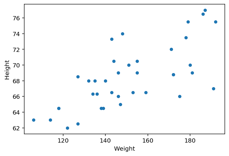
A lot of default ready-to-go Matplotlib plots are available via plot property of Pandas objects:
df.plot.scatter("Weight", "Height")
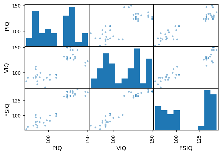
... or in pandas.plotting module:
import matplotlib.pyplot as plt
from pandas import plotting
df_iqs = df[['PIQ', 'VIQ', 'FSIQ']]
plt.figure();
plotting.scatter_matrix(df_iqs);
#plt.show() # Use in script
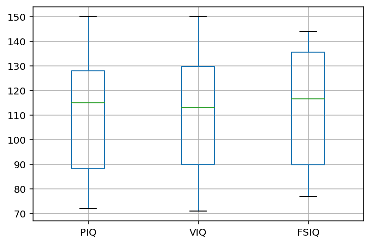
plt.figure();
plotting.boxplot(df_iqs);
#plt.show() # Use in script
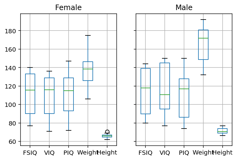
.. or directly on the DataFrameGroupBy objects:
df_bygender.boxplot(column=["FSIQ", "VIQ", "PIQ", "Weight", "Height"])